There are two examples on this page. The first follows here (and is large). The second is under it.
The following Python code contains –
- Using an API to gather labeled data
- The choice of labels can be updated in the code (or the code can be updated to make the labels user-select or froma file)
- Clustering: k-means and hierarchical
- Naive Bayes
- Decision Trees
- Latent Dirchlet Allocation (LDA) – topic modeling
- Several visualizations
NOTE: This is my code 🙂 If you use it, please reference me.
There are three different code examples on this page. Scroll all the way down to see them all.
BELOW – you will find three (3) different Python Code examples for Clustering and related.
## MORE CLUSTERING CODE -
## NOTE - there are many code examples on this page
## scroll to see them all.
##### CLUSTERING -----------------------Gates
##
########################################
##
## Clustering Record and Text Data
##
####################################################
## Gates
####################################################
import nltk
import pandas as pd
import sklearn
from sklearn.cluster import KMeans
import numpy as np
from sklearn.feature_extraction.text import CountVectorizer
from sklearn.feature_extraction.text import TfidfVectorizer
from nltk.tokenize import word_tokenize
from nltk.probability import FreqDist
import matplotlib.pyplot as plt
from nltk.corpus import stopwords
## For Stemming
from nltk.stem import PorterStemmer
from nltk.tokenize import sent_tokenize, word_tokenize
import os
import re ## for regular expressions
from mpl_toolkits.mplot3d import Axes3D
#from nltk.stem.porter import PorterStemmer
####################################################
##
## Clustering Text Data from a Corpus
##
####################################################
## My data and code is here - YOURS IS DIFFERENT
## DATA LINK
# https://drive.google.com/drive/folders/1VSofcdX6g86hjnofMDQJwYVveT544Oy4?usp=sharing
path="C:/Users/profa/Documents/Python Scripts/TextMining/DATA/ClusterCorpus"
## Get the text data first
print("calling os...")
FileNameList=os.listdir(path)
## check the TYPE
print(type(FileNameList))
print(FileNameList)
##-----------
## I need an empty list to start with to build a list of complete paths to files
## Notice that I defined path above. I also need a list of file names.
ListOfCompleteFilePaths=[]
ListOfJustFileNames=[]
for name in os.listdir(path):
## BUILD the names dynamically....
name=name.lower()
print(path+ "/" + name)
next=path+ "/" + name
nextnameL=[re.findall(r'[a-z]+', name)[0]]
nextname=nextnameL[0] ## Keep just the name
print(nextname) ## ALWAYS check yourself
ListOfCompleteFilePaths.append(next)
ListOfJustFileNames.append(nextname)
#print("DONE...")
print("full list...")
print(ListOfCompleteFilePaths)
print(ListOfJustFileNames)
####################################################
## Create the Stemmer Function.........
######################################################
## Instantiate it
A_STEMMER=PorterStemmer()
## test it
print(A_STEMMER.stem("fishers"))
#----------------------------------------
# Use NLTK's PorterStemmer in a function - DEFINE THE FUNCTION
#-------------------------------------------------------
def MY_STEMMER(str_input):
## Only use letters, no punct, no nums, make lowercase...
words = re.sub(r"[^A-Za-z\-]", " ", str_input).lower().split()
words = [A_STEMMER.stem(word) for word in words] ## Use the Stemmer...
return words
##################################################################
## CountVectorizers be set as 'content', 'file', or 'filename'
#If set as ‘filename’, the **sequence passed as an argument to fit**
#is expected to be a list of filenames
#https://scikit-learn.org/stable/modules/generated/
##sklearn.feature_extraction.text.CountVectorizer.html#
##examples-using-sklearn-feature-extraction-text-countvectorizer
##################################################################
## Tokenize and Vectorize the text data from the corpus...
##############################################################
## Instantiate three Vectorizers.....
## NOrmal CV
MyVectCount=CountVectorizer(input='filename',
stop_words='english',
max_features=100
)
## Tf-idf vectorizer
MyVectTFIdf=TfidfVectorizer(input='filename',
stop_words='english',
max_features=100
)
## Create a CountVectorizer object that you can use with the Stemmer
MyCV_Stem = CountVectorizer(input="filename",
stop_words='english',
tokenizer=MY_STEMMER,
lowercase=True)
## NOw I can vectorize using my list of complete paths to my files
DTM_Count=MyVectCount.fit_transform(ListOfCompleteFilePaths)
DTM_TF=MyVectTFIdf.fit_transform(ListOfCompleteFilePaths)
DTM_stem=MyCV_Stem.fit_transform(ListOfCompleteFilePaths)
#####################
## Get the complete vocab - the column names
## !!!!!!!!! FOr TF and CV - but NOT for stemmed...!!!
##################
ColumnNames=MyVectCount.get_feature_names_out()
print("The vocab is: ", ColumnNames, "\n\n")
ColNamesStem=MyCV_Stem.get_feature_names_out()
print("The stemmed vocab is\n", ColNamesStem)
## Use pandas to create data frames
DF_Count=pd.DataFrame(DTM_Count.toarray(),columns=ColumnNames)
DF_TF=pd.DataFrame(DTM_TF.toarray(),columns=ColumnNames)
DF_stem=pd.DataFrame(DTM_stem.toarray(),columns=ColNamesStem)
print(DF_Count)
print(DF_TF.head())
print(DF_stem)
############ --------------->
## OK - now we have vectorized the data - and removed punct, numbers, etc.
## From here, we can update the names of the rows without adding labels
## to the data.
## We CANNOT have labels in the data because:
## 1) Labels are not numeric and (2) Labels are NOT data - they are labels.
#############
## Now update the row names
MyDict={}
for i in range(0, len(ListOfJustFileNames)):
MyDict[i] = ListOfJustFileNames[i]
print("MY DICT:", MyDict)
DF_Count=DF_Count.rename(MyDict, axis="index")
print(DF_Count)
DF_TF=DF_TF.rename(MyDict, axis="index")
print(DF_TF)
## That's pretty!
################################################
## Let's Cluster........
################################################
# Using sklearn
## you will need
## from sklearn.cluster import KMeans
## import numpy as np
kmeans_object_Count = sklearn.cluster.KMeans(n_clusters=2)
#print(kmeans_object)
kmeans_object_Count.fit(DF_Count)
# Get cluster assignment labels
labels = kmeans_object_Count.labels_
prediction_kmeans = kmeans_object_Count.predict(DF_Count)
#print(labels)
print(prediction_kmeans)
# Format results as a DataFrame
Myresults = pd.DataFrame([DF_Count.index,labels]).T
print(Myresults)
############# ---> ALWAYS USE VIS! ----------
print(DF_Count)
print(DF_Count["chocolate"])
x=DF_Count["chocolate"] ## col 1 starting from 0
y=DF_Count["hike"] ## col 14 starting from 0
z=DF_Count["coffee"] ## col 2 starting from 0
colnames=DF_Count.columns
print(colnames)
#print(x,y,z)
fig1 = plt.figure(figsize=(15, 15))
ax1 = fig1.add_subplot(projection='3d')
ax1.scatter(x,y,z, cmap="RdYlGn", edgecolor='k', s=150, c=labels)
ax1.tick_params(axis='both', labelsize=15)
ax1.set_xlabel('Chocolate', fontsize=15)
ax1.set_ylabel('Hike', fontsize=15)
ax1.set_zlabel('Coffee', fontsize=15)
ax1.set_title('Centers and Data')
#
plt.show()
##--------------------------------------
centers = kmeans_object_Count.cluster_centers_
print(centers)
#print(centers)
C1=centers[0,(1,2,14)]
print(C1)
C2=centers[1,(1,2,14)]
print(C2)
xs=C1[0],C2[0]
print(xs)
ys=C1[1],C2[1]
zs=C1[2],C2[2]
ax1.scatter(xs,ys,zs, c='black', s=2000, alpha=0.2)
plt.show()
#plt.cla()
plt.savefig("MyImage1.jpeg")
#---------------- end of choc, dog, hike, example....
#########################################################
##
## kmeans with record data - NEW DATA SETS....
##
##########################################################
##DATA
## https://drive.google.com/file/d/1QtuJO1S-03zDN4f8JgR7cZ1fA3wTZ_m4/view?usp=sharing
##and
## https://drive.google.com/file/d/1sSFzvxkp4wTbna8xAcPBCvInlA_MjNdj/view?usp=sharing
Dataset1="C:/Users/profa/Documents/Python Scripts/TextMining/DATA/ClusterSmallDataset5D.csv"
Dataset2="C:/Users/profa/Documents/Python Scripts/TextMining/DATA/ClusterSmallDataset.csv"
DF5D=pd.read_csv(Dataset1)
DF3D=pd.read_csv(Dataset2)
print(DF3D.head())
print(DF5D.head())
## !!!!!!!!!!!!! This dataset has a label
## We MUST REMOVE IT before we can proceed
TrueLabel3D=DF3D["Label"]
TrueLabel5D=DF5D["Label"]
print(TrueLabel3D)
DF3D=DF3D.drop(['Label'], axis=1) #drop Label, axis = 1 is for columns
DF5D=DF5D.drop(['Label'], axis=1)
print(DF3D.head())
kmeans_object3D = sklearn.cluster.KMeans(n_clusters=2)
kmeans_object5D = sklearn.cluster.KMeans(n_clusters=2)
#print(kmeans_object)
kmeans_3D=kmeans_object3D.fit(DF3D)
kmeans_5D=kmeans_object5D.fit(DF5D)
# Get cluster assignment labels
labels3D =kmeans_3D.labels_
labels5D =kmeans_5D.labels_
prediction_kmeans_3D = kmeans_object3D.predict(DF3D)
prediction_kmeans_5D = kmeans_object5D.predict(DF5D)
print("Prediction 3D\n")
print(prediction_kmeans_3D)
print("Actual\n")
print(TrueLabel3D)
print("Prediction 5D\n")
print(prediction_kmeans_5D)
print("Actual\n")
print(TrueLabel5D)
##---------------------
## Convert True Labels from text to numeric labels...
##-----------------------
print(TrueLabel3D)
data_classes = ["BBallPlayer", "NonPlayer"]
dc = dict(zip(data_classes, range(0,2)))
print(dc)
TrueLabel3D_num=TrueLabel3D.map(dc, na_action='ignore')
print(TrueLabel3D_num)
############# ---> ALWAYS USE VIS! ----------
fig2 = plt.figure(figsize=(15, 15))
ax2 = fig2.add_subplot(projection='3d')
ax2.tick_params(axis='both', labelsize=15)
x=DF3D.iloc[:,0] ## Height
y=DF3D.iloc[:,1] ## Weight
z=DF3D.iloc[:,2] ## Age
print(x,y,z)
ax2.scatter(x,y,z, cmap="RdYlGn", edgecolor='k', s=200, c=prediction_kmeans_3D)
ax2.set_xlabel('Height',fontsize=20)
ax2.set_ylabel('Weight ', fontsize=20)
ax2.set_zlabel('Age', fontsize=20)
ax2.set_title('3D PCA')
#
plt.show()
plt.savefig("MyImage.jpeg")
## These centers should make sense. Notice the actual values....
## The BBPlayers will be taller, higher weight, higher age
centers3D = kmeans_3D.cluster_centers_
print(centers3D)
print(centers3D[0,0])
xs=(centers3D[0,0], centers3D[1,0])
ys=(centers3D[0,1], centers3D[1,1])
zs=(centers3D[0,2], centers3D[1,2])
ax2.scatter(xs,ys,zs, c='black', s=2000, alpha=0.2)
plt.show()
###########################################
## Looking at distances
##############################################
DF3D.head()
## Let's find the distances between each PAIR
## of vectors. What is a vector? It is a data row.
## For example: [84 250 17]
## Where, in this case, 84 is the value for height
## 250 is weight, and 17 is age.
X=DF3D
from sklearn.metrics.pairwise import euclidean_distances
## Distance between each pair of rows (vectors)
Euc_dist=euclidean_distances(X, X)
from sklearn.metrics.pairwise import manhattan_distances
Man_dist=manhattan_distances(X,X)
from sklearn.metrics.pairwise import cosine_distances
Cos_dist=cosine_distances(X,X)
from sklearn.metrics.pairwise import cosine_similarity
Cos_Sim=cosine_similarity(X,X)
#The cosine distance is equivalent to the half the squared
## euclidean distance if each sample is normalized to unit norm
##############-------------------------->
## Visualize distances
################################################
from sklearn.metrics.pairwise import pairwise_distances
from scipy.spatial.distance import squareform
from scipy.cluster.hierarchy import linkage
from scipy.cluster.hierarchy import dendrogram
import numpy as np
import matplotlib.pyplot as plt
import seaborn as sns
print(Euc_dist)
X=DF3D
print(X)
print(type(TrueLabel3D))
## change to list
Labels_3D_asList=list(TrueLabel3D)
print(Labels_3D_asList)
print(type(Labels_3D_asList))
#sns.set() #back to defaults
sns.set(font_scale=3)
Z = linkage(squareform(np.around(euclidean_distances(X), 3)))
fig4 = plt.figure(figsize=(15, 15))
ax4 = fig4.add_subplot(111)
dendrogram(Z, ax=ax4, labels=Labels_3D_asList)
ax4.tick_params(axis='x', which='major', labelsize=15)
ax4.tick_params(axis='y', which='major', labelsize=15)
#ax5 = fig4.add_subplot(212)
fig4.savefig('exampleSave.png')
#######################################
## Normalizing...via scaling MIN MAX
#################################################
## For the heatmap, we must normalize first
#import pandas as pd
from sklearn import preprocessing
x = X.values #returns a numpy array
print(x)
#Instantiate the min-max scaler
min_max_scaler = preprocessing.MinMaxScaler()
x_scaled = min_max_scaler.fit_transform(x)
DF3D_scaled = pd.DataFrame(x_scaled)
print(DF3D.columns)
sns.clustermap(DF3D_scaled,yticklabels=TrueLabel3D,
xticklabels=DF3D.columns)
###############################################
##
## Silhouette and Elbow - Optimal Clusters...
##
#############################################
from sklearn.metrics import silhouette_samples, silhouette_score
#import pandas as pd
#import numpy as np
#import seaborn as sns
#from sklearn.cluster import KMeans
#from sklearn.metrics import silhouette_score
## The Silhouette Method helps to determine the optimal number of clusters
## in kmeans clustering...
#Silhouette Coefficient = (x-y)/ max(x,y)
#where, y is the mean intra cluster distance - the mean distance
## to the other instances in the same cluster.
## x depicts mean nearest cluster distance i.e. the mean distance
## to the instances of the next closest cluster.
## The coefficient varies between -1 and 1.
## A value close to 1 implies that the instance is close to its
## cluster is a part of the right cluster.
## Whereas, a value close to -1 means that the value is
## assigned to the wrong cluster.
#https://scikit-learn.org/stable/auto_examples/cluster/plot_kmeans_silhouette_analysis.html
# The silhouette_score gives the average value for all the samples.
# This gives a perspective into the density and separation of the formed
# clusters
##
## This example is generated from a random mixture of normal data...
## ref:https://towardsdatascience.com/silhouette-coefficient-validating-clustering-techniques-e976bb81d10c
X= np.random.rand(100,2)
print(X)
Y= 2 + np.random.rand(100,2)
Z= np.concatenate((X,Y))
Z=pd.DataFrame(Z)
print(Z.head())
sns.scatterplot(x=Z[0],y=Z[1])
KMean= KMeans(n_clusters=2)
KMean.fit(Z)
label=KMean.predict(Z)
print(label)
#sns.scatterplot(Z[0],Z[1], hue=label)
print("Silhouette Score for k=2\n",silhouette_score(Z, label))
## Now - for k = 3
KMean= KMeans(n_clusters=3)
KMean.fit(Z)
label=KMean.predict(Z)
print("Silhouette Score for k=3\n",silhouette_score(Z, label))
sns.scatterplot(x=Z[0],y=Z[1],hue=label)
## Now - for k = 4
KMean= KMeans(n_clusters=4)
KMean.fit(Z)
label=KMean.predict(Z)
print("Silhouette Score for k=4\n",silhouette_score(Z, label))
sns.scatterplot(x=Z[0],y=Z[1],hue=label)
###############################
## Silhouette Example from sklearn
###################################################
from sklearn.datasets import make_blobs
#from sklearn.cluster import KMeans
#from sklearn.metrics import silhouette_samples, silhouette_score
#import matplotlib.pyplot as plt
import matplotlib.cm as cm
#import numpy as np
X, y = make_blobs(n_samples=500,
n_features=2, ## so it is 2D
centers=4,
cluster_std=1,
center_box=(-10.0, 10.0),
shuffle=True,
random_state=1) # For reproducibility
range_n_clusters = [2, 3, 4, 5, 6]
print(X)
for n_clusters in range_n_clusters:
# Create a subplot with 1 row and 2 columns
fig, (ax1, ax2) = plt.subplots(1, 2)
fig.set_size_inches(18, 7)
# The 1st subplot is the silhouette plot
# The silhouette coefficient can range from -1, 1 but in this example all
# lie within [-0.1, 1]
ax1.set_xlim([-0.1, 1])
# The (n_clusters+1)*10 is for inserting blank space between silhouette
# plots of individual clusters, to demarcate them clearly.
ax1.set_ylim([0, len(X) + (n_clusters + 1) * 10])
# Initialize the clusterer with n_clusters value and a random generator
# seed of 10 for reproducibility.
clusterer = KMeans(n_clusters=n_clusters, random_state=10)
cluster_labels = clusterer.fit_predict(X)
# The silhouette_score gives the average value for all the samples.
# This gives a perspective into the density and separation of the formed
# clusters
silhouette_avg = silhouette_score(X, cluster_labels)
print("For n_clusters =", n_clusters,
"The average silhouette_score is :", silhouette_avg)
# Compute the silhouette scores for each sample
sample_silhouette_values = silhouette_samples(X, cluster_labels)
y_lower = 10
for i in range(n_clusters):
# Aggregate the silhouette scores for samples belonging to
# cluster i, and sort them
ith_cluster_silhouette_values = \
sample_silhouette_values[cluster_labels == i]
ith_cluster_silhouette_values.sort()
size_cluster_i = ith_cluster_silhouette_values.shape[0]
y_upper = y_lower + size_cluster_i
color = cm.nipy_spectral(float(i) / n_clusters)
ax1.fill_betweenx(np.arange(y_lower, y_upper),
0, ith_cluster_silhouette_values,
facecolor=color, edgecolor=color, alpha=0.7)
# Label the silhouette plots with their cluster numbers at the middle
ax1.text(-0.05, y_lower + 0.5 * size_cluster_i, str(i))
# Compute the new y_lower for next plot
y_lower = y_upper + 10 # 10 for the 0 samples
ax1.set_title("The silhouette plot for the various clusters.")
ax1.set_xlabel("The silhouette coefficient values")
ax1.set_ylabel("Cluster label")
# The vertical line for average silhouette score of all the values
ax1.axvline(x=silhouette_avg, color="red", linestyle="--")
ax1.set_yticks([]) # Clear the yaxis labels / ticks
ax1.set_xticks([-0.1, 0, 0.2, 0.4, 0.6, 0.8, 1])
# 2nd Plot showing the actual clusters formed
colors = cm.nipy_spectral(cluster_labels.astype(float) / n_clusters)
ax2.scatter(X[:, 0], X[:, 1], marker='.', s=30, lw=0, alpha=0.7,
c=colors, edgecolor='k')
# Labeling the clusters
centers = clusterer.cluster_centers_
# Draw white circles at cluster centers
ax2.scatter(centers[:, 0], centers[:, 1], marker='o',
c="white", alpha=1, s=200, edgecolor='k')
for i, c in enumerate(centers):
ax2.scatter(c[0], c[1], marker='$%d$' % i, alpha=1,
s=50, edgecolor='k')
ax2.set_title("The visualization of the clustered data.")
ax2.set_xlabel("Feature space for the 1st feature")
ax2.set_ylabel("Feature space for the 2nd feature")
plt.suptitle(("Silhouette analysis for KMeans clustering on sample data "
"with n_clusters = %d" % n_clusters),
fontsize=14, fontweight='bold')
plt.show()
## References:
#https://ncss-wpengine.netdna-ssl.com/wp-content/themes/ncss/pdf/Procedures/NCSS/Hierarchical_Clustering-Dendrograms.pdf
###### Overview of distances reference....
#'minkowski', 'cityblock', 'cosine', 'correlation',
# 'hamming', 'jaccard', 'chebyshev', 'canberra',
## 'mahalanobis', VI=None...
## RE: https://docs.scipy.org/doc/scipy/reference/generated/scipy.spatial.distance.pdist.html#scipy.spatial.distance.pdist
------------------------------------------------------------------------------------
# -*- coding: utf-8 -*-
"""
Created on Sun Feb 9 13:23:28 2025
@author: profa
"""
########################################
## Gates
##
## Topics:
# Data gathering via API
# - URLs and GET
# Cleaning and preparing text DATA
# DTM and Data Frames
# Training and Testing at DT
# CLustering
## LDA
#########################################
## ATTENTION READER...
##
## First, you will need to go to
## https://newsapi.org/
## https://newsapi.org/register
## and get an API key
################## DO NOT USE MY KEY!!
## Get your own key.
##
###################################################
### API KEY - get a key!
##https://newsapi.org/
## Example URL
## https://newsapi.org/v2/everything?
## q=tesla&from=2021-05-20&sortBy=publishedAt&
## apiKey=YOUR KEY HERE
## !!
## YOU CAN FIND THIS CODE
## HERE
## https://gatesboltonanalytics.com/?page_id=1114
##!!
## What to import
import requests ## for getting data from a server
import re ## for regular expressions
import pandas as pd ## for dataframes and related
from pandas import DataFrame
## To tokenize and vectorize text type data
from sklearn.feature_extraction.text import CountVectorizer
import numpy as np
## For word clouds
## conda install -c conda-forge wordcloud
## May also have to run conda update --all on cmd
#import PIL
#import Pillow
#import wordcloud
from wordcloud import WordCloud, STOPWORDS
import matplotlib.pyplot as plt
from sklearn.model_selection import train_test_split
import random as rd
from sklearn.naive_bayes import MultinomialNB
from sklearn.metrics import confusion_matrix
#from sklearn.naive_bayes import BernoulliNB
from sklearn.tree import DecisionTreeClassifier, plot_tree
from sklearn import tree
## conda install python-graphviz
## restart kernel (click the little red x next to the Console)
import graphviz
from sklearn.decomposition import LatentDirichletAllocation
import matplotlib.pyplot as plt
import numpy as np
from sklearn.metrics import silhouette_samples, silhouette_score
import sklearn
from sklearn.cluster import KMeans
from sklearn import preprocessing
import seaborn as sns
import numpy as np
import pandas as pd
from sklearn.metrics.pairwise import euclidean_distances
from sklearn.metrics.pairwise import cosine_similarity
import matplotlib.pyplot as plt
from sklearn.manifold import MDS
from mpl_toolkits.mplot3d import Axes3D
from scipy.cluster.hierarchy import ward, dendrogram
####################################
##
## Step 1: Connect to the server
## Send a query
## Collect and clean the
## results
####################################
####################################################
##In the following loop, we will query thenewsapi servers
##for all the topic names in the list
## We will then build a large csv file
## where each article is a row
##
## From there, we will convert this data
## into a labeled dataframe
## so we can train and then test our DT
## model
####################################################
####################################################
## Build the URL and GET the results
## NOTE: At the bottom of this code
## commented out, you will find a second
## method for doing the following. This is FYI.
####################################################
## This is the endpoint - the server and
## location on the server where your data
## will be retrieved from
## TEST FIRST!
## We are about to build this URL:
## https://newsapi.org/v2/everything?apiKey=YourKeyHere&q=bitcoin
##Any topics you want and however many topics you want....
topics=["politics", "food", "business", "sports", "pets"]
## topics needs to be a list of strings (words)
## Next, let's build the csv file
## first and add the column names
## Create a new csv file to save the headlines
filename="NewHeadlines.csv"
MyFILE=open(filename,"w")
### Place the column names in - write to the first row
WriteThis="LABEL,Date,Source,Title,Headline\n"
MyFILE.write(WriteThis)
MyFILE.close()
## CHeck it! Can you find this file?
#### --------------------> GATHER - CLEAN - CREATE FILE
## RE: documentation and options
## https://newsapi.org/docs/endpoints/everything
endpoint="https://newsapi.org/v2/everything"
################# enter for loop to collect
################# data on three topics
#######################################
for topic in topics:
## Dictionary Structure
URLPost = {'apiKey':'yourkeyhere',
'q':topic,
'language':'en'}
response=requests.get(endpoint, URLPost)
print(response)
jsontxt = response.json()
print(jsontxt)
#####################################################
## Open the file for append
MyFILE=open(filename, "a")
LABEL=topic
for items in jsontxt["articles"]:
print(items, "\n\n\n")
#Author=items["author"]
#Author=str(Author)
#Author=Author.replace(',', '')
Source=items["source"]["id"]
print(Source)
Date=items["publishedAt"]
##clean up the date
NewDate=Date.split("T")
Date=NewDate[0]
print(Date)
## CLEAN the Title
##----------------------------------------------------------
##Replace punctuation with space
# Accept one or more copies of punctuation
# plus zero or more copies of a space
# and replace it with a single space
Title=items["title"]
Title=str(Title)
#print(Title)
Title=re.sub(r'[,.;@#?!&$\-\']+', ' ', str(Title), flags=re.IGNORECASE)
Title=re.sub(' +', ' ', str(Title), flags=re.IGNORECASE)
Title=re.sub(r'\"', ' ', str(Title), flags=re.IGNORECASE)
print(Title)
# and replace it with a single space
## NOTE: Using the "^" on the inside of the [] means
## we want to look for any chars NOT a-z or A-Z and replace
## them with blank. This removes chars that should not be there.
Title=re.sub(r'[^a-zA-Z]', " ", str(Title), flags=re.VERBOSE)
Title=Title.replace(',', '')
Title=' '.join(Title.split())
Title=re.sub("\n|\r", "", Title)
##----------------------------------------------------------
Headline=items["description"]
Headline=str(Headline)
Headline=re.sub(r'[,.;@#?!&$\-\']+', ' ', Headline, flags=re.IGNORECASE)
Headline=re.sub(' +', ' ', Headline, flags=re.IGNORECASE)
Headline=re.sub(r'\"', ' ', Headline, flags=re.IGNORECASE)
Headline=re.sub(r'[^a-zA-Z]', " ", Headline, flags=re.VERBOSE)
## Be sure there are no commas in the headlines or it will
## write poorly to a csv file....
Headline=Headline.replace(',', '')
Headline=' '.join(Headline.split())
Headline=re.sub("\n|\r", "", Headline)
### AS AN OPTION - remove words of a given length............
Headline = ' '.join([wd for wd in Headline.split() if len(wd)>3])
#print("Author: ", Author, "\n")
#print("Title: ", Title, "\n")
#print("Headline News Item: ", Headline, "\n\n")
#print(Author)
print(Title)
print(Headline)
WriteThis=str(LABEL)+","+str(Date)+","+str(Source)+","+ str(Title) + "," + str(Headline) + "\n"
MyFILE.write(WriteThis)
## CLOSE THE FILE
MyFILE.close()
################## END for loop
####################################################
##
## Where are we now?
##
## So far, we have created a csv file
## with labeled data. Each row is a news article
##
## - BUT -
## We are not done. We need to choose which
## parts of this data to use to model our decision tree
## and we need to convert the data into a data frame.
##
########################################################
BBC_DF=pd.read_csv(filename)
print(BBC_DF.head())
# iterating the columns
for col in BBC_DF.columns:
print(col)
print(BBC_DF["Headline"])
## REMOVE any rows with NaN in them
BBC_DF = BBC_DF.dropna()
print(BBC_DF["Headline"])
### Tokenize and Vectorize the Headlines
## Create the list of headlines
## Keep the labels!
HeadlineLIST=[]
LabelLIST=[]
for nexthead, nextlabel in zip(BBC_DF["Headline"], BBC_DF["LABEL"]):
HeadlineLIST.append(nexthead)
LabelLIST.append(nextlabel)
print("The headline list is:\n")
print(HeadlineLIST)
print("The label list is:\n")
print(LabelLIST)
##########################################
## Remove all words that match the topics.
## For example, if the topics are food and covid
## remove these exact words.
##
## We will need to do this by hand.
NewHeadlineLIST=[]
for element in HeadlineLIST:
print(element)
print(type(element))
## make into list
AllWords=element.split(" ")
print(AllWords)
## Now remove words that are in your topics
NewWordsList=[]
for word in AllWords:
print(word)
word=word.lower()
if word in topics:
print(word)
else:
NewWordsList.append(word)
##turn back to string
NewWords=" ".join(NewWordsList)
## Place into NewHeadlineLIST
NewHeadlineLIST.append(NewWords)
##
## Set the HeadlineLIST to the new one
HeadlineLIST=NewHeadlineLIST
print(HeadlineLIST)
#########################################
##
## Build the labeled dataframe
##
######################################################
### Vectorize
## Instantiate your CV
MyCountV=CountVectorizer(
input="content", ## because we have a csv file
lowercase=True,
stop_words = "english",
max_features=50
)
## Use your CV
MyDTM = MyCountV.fit_transform(HeadlineLIST) # create a sparse matrix
print(type(MyDTM))
ColumnNames=MyCountV.get_feature_names_out()
#print(type(ColumnNames))
## Build the data frame
MyDTM_DF=pd.DataFrame(MyDTM.toarray(),columns=ColumnNames)
## Convert the labels from list to df
Labels_DF = DataFrame(LabelLIST,columns=['LABEL'])
## Check your new DF and you new Labels df:
print("Labels\n")
print(Labels_DF)
print("News df\n")
print(MyDTM_DF.iloc[:,0:6])
##Save original DF - without the lables
My_Orig_DF=MyDTM_DF
print(My_Orig_DF)
######################
## AND - just to make sure our dataframe is fair
## let's remove columns called:
## food, bitcoin, and sports (as these are label names)
######################
#MyDTM_DF=MyDTM_DF.drop(topics, axis=1)
## Now - let's create a complete and labeled
## dataframe:
dfs = [Labels_DF, MyDTM_DF]
Final_News_DF_Labeled = pd.concat(dfs,axis=1, join='inner')
## DF with labels
print(Final_News_DF_Labeled)
#############################################
##
## Create Training and Testing Data
##
## Then model and test the Decision Tree
##
################################################
## Before we start our modeling, let's visualize and
## explore.
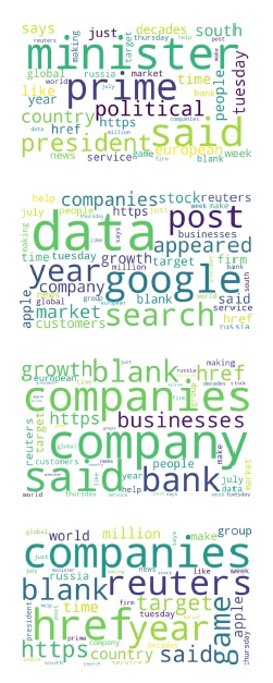
##It might be very interesting to see the word clouds
## for each of the topics.
##--------------------------------------------------------
List_of_WC=[]
for mytopic in topics:
tempdf = Final_News_DF_Labeled[Final_News_DF_Labeled['LABEL'] == mytopic]
print(tempdf)
tempdf =tempdf.sum(axis=0,numeric_only=True)
#print(tempdf)
#Make var name
NextVarName=str("wc"+str(mytopic))
#print( NextVarName)
##In the same folder as this code, I have three images
## They are called: food.jpg, bitcoin.jpg, and sports.jpg
#next_image=str(str(mytopic) + ".jpg")
#print(next_image)
## https://amueller.github.io/word_cloud/generated/wordcloud.WordCloud.html
###########
## Create and store in a list the wordcloud OBJECTS
#########
NextVarName = WordCloud(width=1000, height=600, background_color="white",
min_word_length=4, #mask=next_image,
max_words=200).generate_from_frequencies(tempdf)
## Here, this list holds all three wordclouds I am building
List_of_WC.append(NextVarName)
##------------------------------------------------------------------
print(List_of_WC)
##########
########## Create the wordclouds
##########
fig=plt.figure(figsize=(25, 25))
#figure, axes = plt.subplots(nrows=2, ncols=2)
NumTopics=len(topics)
for i in range(NumTopics):
print(i)
ax = fig.add_subplot(NumTopics,1,i+1)
plt.imshow(List_of_WC[i], interpolation='bilinear')
plt.axis("off")
plt.savefig("NewClouds.pdf")
###########################################################
##
##
## Clustering
##
##
############################################################
## Our DF
print(My_Orig_DF)
#from sklearn.metrics import silhouette_samples, silhouette_score
#from sklearn.cluster import KMeans
My_KMean= KMeans(n_clusters=3)
My_KMean.fit(My_Orig_DF)
My_labels=My_KMean.predict(My_Orig_DF)
print(My_labels)
#from sklearn import preprocessing
#from sklearn.cluster import KMeans
#import seaborn as sns
My_KMean2 = KMeans(n_clusters=4).fit(preprocessing.normalize(My_Orig_DF))
My_KMean2.fit(My_Orig_DF)
My_labels2=My_KMean2.predict(My_Orig_DF)
print(My_labels2)
My_KMean3= KMeans(n_clusters=3)
My_KMean3.fit(My_Orig_DF)
My_labels3=My_KMean3.predict(My_Orig_DF)
print("Silhouette Score for k = 3 \n",silhouette_score(My_Orig_DF, My_labels3))
#https://docs.scipy.org/doc/scipy/reference/generated/scipy.cluster.hierarchy.linkage.html
#length of the document: called cosine similarity
print(len(My_Orig_DF))
cosdist = 1 - cosine_similarity(My_Orig_DF)
print(cosdist)
print(len(cosdist))
print(np.round(cosdist,3)) #cos dist should be .02
#----------------------------------------------------------
## Hierarchical Clustering using ward and cosine sim
labels=list(Final_News_DF_Labeled["LABEL"])
print(labels)
print(len(labels))
print(type(labels))
linkage_matrix = ward(cosdist) #define the linkage_matrix
#using ward clustering pre-computed distances
print(linkage_matrix)
print(len(linkage_matrix))
fig = plt.figure(figsize=(25, 10))
dn = dendrogram(linkage_matrix, labels=labels, leaf_rotation=90)
plt.show()
###############################################################
##
## Model with two ML supervised options
##
## DT
## NB (multinomial)
##
###############################################################
## STEP 1 Create Training and Testing Data
###############################################################
## Write the dataframe to csv so you can use it later if you wish
##
Final_News_DF_Labeled.to_csv("Labeled_News_Data_from_API.csv")
TrainDF, TestDF = train_test_split(Final_News_DF_Labeled, test_size=0.3)
print(TrainDF)
print(TestDF)
#################################################
## STEP 2: Separate LABELS
#################################################
## IMPORTANT - YOU CANNOT LEAVE LABELS ON
## Save labels
### TEST ---------------------
TestLabels=TestDF["LABEL"]
print(TestLabels)
TestDF = TestDF.drop(["LABEL"], axis=1)
print(TestDF)
### TRAIN----------------------
TrainLabels=TrainDF["LABEL"]
print(TrainLabels)
## remove labels
TrainDF = TrainDF.drop(["LABEL"], axis=1)
##################################################
## STEP 3: Run MNB
##################################################
## Instantiate
MyModelNB= MultinomialNB()
## FIT
MyNB=MyModelNB.fit(TrainDF, TrainLabels)
#print(MyNB.classes_)
#print(MyNB.class_count_)
#print(MyNB.feature_log_prob_)
Prediction = MyModelNB.predict(TestDF)
print(np.round(MyModelNB.predict_proba(TestDF),2))
## COnfusion Matrix Accuracies
cnf_matrix = confusion_matrix(TestLabels, Prediction)
print("\nThe confusion matrix is:")
print(cnf_matrix)
##################################################
## STEP 3: Run DT
##################################################
## Instantiate
MyDT=DecisionTreeClassifier(criterion='entropy', ##"entropy" or "gini"
splitter='best', ## or "random" or "best"
max_depth=None,
min_samples_split=2,
min_samples_leaf=1,
min_weight_fraction_leaf=0.0,
max_features=None,
random_state=None,
max_leaf_nodes=None,
min_impurity_decrease=0.0,
class_weight=None)
##
MyDT.fit(TrainDF, TrainLabels)
print(ColumnNames)
print(len(ColumnNames))
print(Labels_DF)
print(type(Labels_DF))
## Convert to LIST
Labels_DF_List = Labels_DF["LABEL"].to_list()
print(Labels_DF_List)
print(type(Labels_DF_List))
print(len(Labels_DF_List))
plt.figure(figsize=(50,30))
plot_tree(MyDT, feature_names=ColumnNames,
class_names=Labels_DF_List,
filled=True,
#max_depth=5,
fontsize=10)
plt.show()
# If saving the figure is needed:
plt.savefig("decision_tree.jpeg")
## COnfusion Matrix
print("Prediction\n")
DT_pred=MyDT.predict(TestDF)
print(DT_pred)
bn_matrix = confusion_matrix(TestLabels, DT_pred)
print("\nThe confusion matrix is:")
print(bn_matrix)
feature_names=ColumnNames
FeatureImp=MyDT.feature_importances_
indices = np.argsort(FeatureImp)[::-1]
## print out the important features.....
for f in range(TrainDF.shape[1]):
if FeatureImp[indices[f]] > 0:
print("%d. feature %d (%f)" % (f + 1, indices[f], FeatureImp[indices[f]]))
print ("feature name: ", feature_names[indices[f]])
##############################################
##
## LDA Topics Modeling
##
##
#########################################################
NUM_TOPICS=NumTopics
lda_model = LatentDirichletAllocation(n_components=NUM_TOPICS, max_iter=10000, learning_method='online')
#lda_model = LatentDirichletAllocation(n_components=NUM_TOPICS, max_iter=10, learning_method='online')
lda_Z_DF = lda_model.fit_transform(My_Orig_DF)
print(lda_Z_DF.shape) # (NO_DOCUMENTS, NO_TOPICS)
def print_topics(model, vectorizer, top_n=10):
for idx, topic in enumerate(model.components_):
print("Topic %d:" % (idx))
print([(vectorizer.get_feature_names_out()[i], topic[i])
for i in topic.argsort()[:-top_n - 1:-1]])
print("LDA Model:")
print_topics(lda_model, MyCountV)
################ Another fun vis for LDA
plt.figure(figsize=(50,30))
word_topic = np.array(lda_model.components_)
#print(word_topic)
word_topic = word_topic.transpose()
num_top_words = 15
vocab_array = np.asarray(ColumnNames)
#fontsize_base = 70 / np.max(word_topic) # font size for word with largest share in corpus
fontsize_base = 40
for t in range(NUM_TOPICS):
plt.subplot(1, NUM_TOPICS, t + 1) # plot numbering starts with 1
plt.ylim(0, num_top_words + 0.5) # stretch the y-axis to accommodate the words
plt.xticks([]) # remove x-axis markings ('ticks')
plt.yticks([]) # remove y-axis markings ('ticks')
plt.title('Topic #{}'.format(t))
top_words_idx = np.argsort(word_topic[:,t])[::-1] # descending order
top_words_idx = top_words_idx[:num_top_words]
top_words = vocab_array[top_words_idx]
top_words_shares = word_topic[top_words_idx, t]
for i, (word, share) in enumerate(zip(top_words, top_words_shares)):
plt.text(0.3, num_top_words-i-0.5, word, fontsize=fontsize_base/2)
##fontsize_base*share)
plt.savefig("TopicsVis.pdf")
plt.show()
#############################################
## Silhouette and clusters
#############################################
#from sklearn.metrics import silhouette_samples, silhouette_score
## Using MyDTM_DF which is not labeled
# =============================================================================
# KMean= KMeans(n_clusters=3)
# KMean.fit(MyDTM_DF)
# label=KMean.predict(MyDTM_DF)
# print(label)
#
# #sns.scatterplot(MyDTM_DF[0],MyDTM_DF[1], hue=label)
# print("Silhouette Score for k=3\n",silhouette_score(MyDTM_DF, label))
# #
# =============================================================================
##############################
## Check These files now on your computer...
#############################################
## NewClouds.pdf
## TopicsVis.pdf
## InTheNews.html
## Labeled_News_Data_from_API.csv
The following code shows many examples of text and record data connected to Clustering and other methods.

########################################
##
## Clustering Record and Text Data
##
####################################################
## Gates
####################################################

import nltk
import pandas as pd
import sklearn
from sklearn.cluster import KMeans
import numpy as np
from sklearn.feature_extraction.text import CountVectorizer
from sklearn.feature_extraction.text import TfidfVectorizer
from nltk.tokenize import word_tokenize
from nltk.probability import FreqDist
import matplotlib.pyplot as plt
from nltk.corpus import stopwords
## For Stemming
from nltk.stem import PorterStemmer
from nltk.tokenize import sent_tokenize, word_tokenize
import os
import re   ## for regular expressions
#from mpl_toolkits.mplot3d import Axes3D
#from nltk.stem.porter import PorterStemmer

####################################################
##
##  Clustering Text Data from a Corpus
##
####################################################
## My data and code is here - YOURS IS DIFFERENT
## DATA LINK
# https://drive.google.com/drive/folders/1VSofcdX6g86hjnofMDQJwYVveT544Oy4?usp=sharing
path="C:/Users/profa/Documents/Python Scripts/TextMining/DATA/ClusterCorpus"

## Get the text data first
print("calling os...")
FileNameList=os.listdir(path)
## check the TYPE
print(type(FileNameList))
print(FileNameList)

##-----------
## I need an empty list to start with to build a list of complete paths to files
## Notice that I defined path above. I also need a list of file names.
ListOfCompleteFilePaths=[]
ListOfJustFileNames=[]

for name in os.listdir(path):
    ## BUILD the names dynamically....
    name=name.lower()
    print(path+ "/" + name)
    next=path+ "/" + name

    nextnameL=[re.findall(r'[a-z]+', name)[0]]
    nextname=nextnameL[0]   ## Keep just the name
    print(nextname)  ## ALWAYS check yourself

    ListOfCompleteFilePaths.append(next)
    ListOfJustFileNames.append(nextname)

#print("DONE...")
print("full list...")
print(ListOfCompleteFilePaths)
print(ListOfJustFileNames)

####################################################
##  Create the Stemmer Function.........
######################################################
## Instantiate it
A_STEMMER=PorterStemmer()
## test it
print(A_STEMMER.stem("fishers"))
#----------------------------------------
# Use NLTK's PorterStemmer in a function - DEFINE THE FUNCTION
#-------------------------------------------------------
def MY_STEMMER(str_input):
    ## Only use letters, no punct, no nums, make lowercase...
    words = re.sub(r"[^A-Za-z\-]", " ", str_input).lower().split()
    print(words)
    words = [A_STEMMER.stem(word) for word in words] ## Use the Stemmer...
    return words


##################################################################
## CountVectorizers be set as 'content', 'file', or 'filename'
        #If set as ‘filename’, the **sequence passed as an argument to fit**
        #is expected to be a list of filenames
        #https://scikit-learn.org/stable/modules/generated/
        ##sklearn.feature_extraction.text.CountVectorizer.html#
        ##examples-using-sklearn-feature-extraction-text-countvectorizer

##################################################################
## Tokenize and Vectorize the text data from the corpus...
##############################################################
## Instantiate three Vectorizers.....
## NOrmal CV
MyVectCount=CountVectorizer(input='filename',   ## 'content'
                        stop_words='english',  ## and, of, the, is, ...
                        max_features=100
                        )
## Tf-idf vectorizer
MyVectTFIdf=TfidfVectorizer(input='filename',
                        stop_words='english',
                        max_features=100
                        )

## Create a CountVectorizer object that you can use with the Stemmer
MyCV_Stem = CountVectorizer(input="filename",
                        stop_words='english',
                        tokenizer=MY_STEMMER, ## hikes and hike --> one col hik
                        lowercase=True)


## NOw I can vectorize using my list of complete paths to my files
DTM_Count=MyVectCount.fit_transform(ListOfCompleteFilePaths)
DTM_TF=MyVectTFIdf.fit_transform(ListOfCompleteFilePaths)
DTM_stem=MyCV_Stem.fit_transform(ListOfCompleteFilePaths)

#####################
## Get the complete vocab - the column names
## !!!!!!!!! FOr TF and CV - but NOT for stemmed...!!!
##################
ColumnNames=MyVectCount.get_feature_names_out()
print("The vocab is: ", ColumnNames, "\n\n")
ColNamesStem=MyCV_Stem.get_feature_names_out()
print("The stemmed vocab is\n", ColNamesStem)

## Use pandas to create data frames
DF_Count=pd.DataFrame(DTM_Count.toarray(),columns=ColumnNames)
DF_TF=pd.DataFrame(DTM_TF.toarray(),columns=ColumnNames)
DF_stem=pd.DataFrame(DTM_stem.toarray(),columns=ColNamesStem)
print(DF_Count)
print(DF_TF)
print(DF_stem)

############ --------------->
## OK - now we have vectorized the data - and removed punct, numbers, etc.
## From here, we can update the names of the rows without adding labels
## to the data.
## We CANNOT have labels in the data because:
## 1) Labels are not numeric and (2) Labels are NOT data - they are labels.
#############

## Now update the row names
MyDict={}
for i in range(0, len(ListOfJustFileNames)):
    MyDict[i] = ListOfJustFileNames[i]

print("MY DICT:", MyDict)

DF_Count=DF_Count.rename(MyDict, axis="index")
print(DF_Count)

DF_TF=DF_TF.rename(MyDict, axis="index")
print(DF_TF)
## That's pretty!

################################################
##           Let's Cluster........
################################################
# Using sklearn
## you will need
## from sklearn.cluster import KMeans
## import numpy as np
kmeans_object_Count = sklearn.cluster.KMeans(n_clusters=2, init="random")
#print(kmeans_object)
kmeans_object_Count.fit(DF_Count)
# Get cluster assignment labels
labels = kmeans_object_Count.labels_
prediction_kmeans = kmeans_object_Count.predict(DF_Count)
#print(labels)
print(prediction_kmeans)
# Format results as a DataFrame
Myresults = pd.DataFrame([DF_Count.index,labels]).T
print(Myresults)

Centers=kmeans_object_Count.cluster_centers_
print(Centers)
print(Centers.shape)

############# ---> ALWAYS USE VIS! ----------
print(DF_Count)
print(DF_Count["chocolate"])
x=DF_Count["chocolate"]  ## col 1  starting from 0
y=DF_Count["hike"]    ## col 14  starting from 0
z=DF_Count["coffee"]  ## col 2  starting from 0
colnames=DF_Count.columns
print(colnames)
#print(x,y,z)
fig1 = plt.figure(figsize=(12, 12))
ax1 = fig1.add_subplot(projection='3d')
ax1.scatter(x,y,z, cmap="RdYlGn", edgecolor='k', s=200,c=prediction_kmeans)
ax1.set_xlim(-10, 10)
ax1.set_ylim(-10, 10)
ax1.set_zlim(-10, 10)

ax1.set_xlabel('Chocolate', fontsize=10)
ax1.set_ylabel('Hike', fontsize=10)
ax1.set_zlabel('Coffee', fontsize=10)
#plt.show()

centers = kmeans_object_Count.cluster_centers_
print(centers)
#print(centers)
C1=centers[0,(1,2,14)]
print(C1)
C2=centers[1,(1,2,14)]
print(C2)
xs=C1[0],C2[0]
print(xs)
ys=C1[1],C2[1]
zs=C1[2],C2[2]


ax1.scatter(xs,ys,zs, c='black', s=2000, alpha=0.2)
plt.show()
#plt.cla()

#---------------- end of choc, dog, hike, example....

#########################################################
##
##     kmeans with record data - NEW DATA SETS....
##
##########################################################

##DATA
## https://drive.google.com/file/d/1QtuJO1S-03zDN4f8JgR7cZ1fA3wTZ_m4/view?usp=sharing
##and
## https://drive.google.com/file/d/1sSFzvxkp4wTbna8xAcPBCvInlA_MjNdj/view?usp=sharing

Dataset1="C:/Users/profa/Documents/Python Scripts/TextMining/DATA/ClusterSmallDataset5D.csv"
Dataset2="C:/Users/profa/Documents/Python Scripts/TextMining/DATA/ClusterSmallDataset.csv"

DF5D=pd.read_csv(Dataset1)
DF3D=pd.read_csv(Dataset2)

print(DF3D.head())
print(DF5D.head())


## !!!!!!!!!!!!! This dataset has a label
## We MUST REMOVE IT before we can proceed
TrueLabel3D=DF3D["Label"]
TrueLabel5D=DF5D["Label"]
print(TrueLabel3D)

DF3D=DF3D.drop(['Label'], axis=1) #drop Label, axis = 1 is for columns
DF5D=DF5D.drop(['Label'], axis=1)

print(DF3D.head())

kmeans_object3D = sklearn.cluster.KMeans(n_clusters=2)
kmeans_object5D = sklearn.cluster.KMeans(n_clusters=2)

#print(kmeans_object)
kmeans_3D=kmeans_object3D.fit(DF3D)
kmeans_5D=kmeans_object5D.fit(DF5D)
# Get cluster assignment labels
labels3D =kmeans_3D.labels_
labels5D =kmeans_5D.labels_

prediction_kmeans_3D = kmeans_object3D.predict(DF3D)
prediction_kmeans_5D = kmeans_object5D.predict(DF5D)

print("Prediction 3D\n")
print(prediction_kmeans_3D)
print("Actual\n")
print(TrueLabel3D)

print("Prediction 5D\n")
print(prediction_kmeans_5D)
print("Actual\n")
print(TrueLabel5D)

##---------------------
## Convert True Labels from text to numeric labels...
##-----------------------
print(TrueLabel3D)
data_classes = ["BBallPlayer", "NonPlayer"]
dc = dict(zip(data_classes, range(0,2)))
print(dc)
TrueLabel3D_num=TrueLabel3D.map(dc, na_action='ignore')
print(TrueLabel3D_num)


############# ---> ALWAYS USE VIS! ----------

fig2 = plt.figure()
    #figsize=(12, 12))
ax2 = fig2.add_subplot(projection='3d')
## Use the SAME axis values so you can SEE the shift!
#ax2.set_xlim(-10, 10)
#ax2.set_ylim(-10, 10)
#ax2.set_zlim(-10, 10)

print(DF3D)
x=DF3D.iloc[:,0] ## Height
y=DF3D.iloc[:,1] ## Weight
z=DF3D.iloc[:,2] ## Age
print(x,y,z)

ax2.scatter(x,y,z, cmap="RdYlGn", edgecolor='k', s=200,c=prediction_kmeans_3D)

ax2.set_xlabel('Height', fontsize=15)
ax2.set_ylabel('Weight', fontsize=15)
ax2.set_zlabel('Age', fontsize=15)
#
plt.show()

## These centers should make sense. Notice the actual values....
## The BBPlayers will be taller, higher weight, higher age
centers3D = kmeans_3D.cluster_centers_
print(centers3D)
print(centers3D[0,0])
xs=(centers3D[0,0], centers3D[1,0])
ys=(centers3D[0,1], centers3D[1,1])
zs=(centers3D[0,2], centers3D[1,2])


ax2.scatter(xs,ys,zs, c='black', s=2000, alpha=0.2)
plt.show()

plt.savefig("Clustering_Centroids.jpeg")


###########################################
## Looking at distances
##############################################
DF3D.head()

## Let's find the distances between each PAIR
## of vectors. What is a vector? It is a data row.
## For example:  [84       250         17]
## Where, in this case, 84 is the value for height
## 250 is weight, and 17 is age.

X=DF3D

from sklearn.metrics.pairwise import euclidean_distances
## Distance between each pair of rows (vectors)
Euc_dist=euclidean_distances(X, X)
print(Euc_dist)

from sklearn.metrics.pairwise import manhattan_distances
Man_dist=manhattan_distances(X,X)
print(Man_dist)

from sklearn.metrics.pairwise import cosine_distances
Cos_dist=cosine_distances(X,X)
print(Cos_dist)

from sklearn.metrics.pairwise import cosine_similarity
Cos_Sim=cosine_similarity(X,X)
print(Cos_Sim)

#The cosine distance is equivalent to the half the squared
## euclidean distance if each sample is normalized to unit norm

##############-------------------------->
## Visualize distances
################################################
from sklearn.metrics.pairwise import pairwise_distances
from scipy.spatial.distance import squareform
from scipy.cluster.hierarchy import linkage
from scipy.cluster.hierarchy import dendrogram
import numpy as np
import matplotlib.pyplot as plt
import seaborn as sns

print(Euc_dist)
X=DF3D
#sns.set()  #back to defaults
sns.set(font_scale=3)
Z = linkage(squareform(np.around(euclidean_distances(X), 3)))

fig4 = plt.figure(figsize=(15, 15))
ax4 = fig4.add_subplot(111)
dendrogram(Z, ax=ax4)
ax4.tick_params(axis='x', which='major', labelsize=15)
ax4.tick_params(axis='y', which='major', labelsize=15)
#ax5 = fig4.add_subplot(212)
fig4.savefig('exampleSave.png')

#######################################
## Normalizing...via scaling MIN MAX
#################################################
## For the heatmap, we must normalize first
#import pandas as pd
from sklearn import preprocessing

x = X.values #returns a numpy array
print(x)
#Instantiate the min-max scaler
min_max_scaler = preprocessing.MinMaxScaler()
x_scaled = min_max_scaler.fit_transform(x)
DF3D_scaled = pd.DataFrame(x_scaled)
print(DF3D.columns)
sns.clustermap(DF3D_scaled,yticklabels=TrueLabel3D,
               xticklabels=DF3D.columns)


###############################################
##
##   Silhouette and Elbow - Optimal Clusters...
##
#############################################
from sklearn.metrics import silhouette_samples, silhouette_score

#import pandas as pd
#import numpy as np
#import seaborn as sns
#from sklearn.cluster import KMeans
#from sklearn.metrics import silhouette_score

## The Silhouette Method helps to determine the optimal number of clusters
    ## in kmeans clustering...

    #Silhouette Coefficient = (x-y)/ max(x,y)

    #where, y is the mean intra cluster distance - the mean distance
    ## to the other instances in the same cluster.
    ## x depicts mean nearest cluster distance i.e. the mean distance
    ## to the instances of the next closest cluster.
    ## The coefficient varies between -1 and 1.
    ## A value close to 1 implies that the instance is close to its
    ## cluster is a part of the right cluster.
    ## Whereas, a value close to -1 means that the value is
    ## assigned to the wrong cluster.

#https://scikit-learn.org/stable/auto_examples/cluster/plot_kmeans_silhouette_analysis.html
# The silhouette_score gives the average value for all the samples.
    # This gives a perspective into the density and separation of the formed
    # clusters

##
    ## This example is generated from a random mixture of normal data...
    ## ref:https://towardsdatascience.com/silhouette-coefficient-validating-clustering-techniques-e976bb81d10c
X= np.random.rand(100,2)
print(X)
Y= 2 + np.random.rand(100,2)
Z= np.concatenate((X,Y))
Z=pd.DataFrame(Z)
print(Z.head())

sns.scatterplot(x=Z[0],y=Z[1])

KMean= KMeans(n_clusters=2)
KMean.fit(Z)
label=KMean.predict(Z)
print(label)

sns.scatterplot(x=Z[0],y=Z[1], hue=label)
print("Silhouette Score for k=2\n",silhouette_score(Z, label))


## Now - for k = 3
KMean= KMeans(n_clusters=3)
KMean.fit(Z)
label=KMean.predict(Z)
print("Silhouette Score for k=3\n",silhouette_score(Z, label))
sns.scatterplot(x=Z[0],y=Z[1],hue=label)

## Now - for k = 4
KMean= KMeans(n_clusters=4)
KMean.fit(Z)
label=KMean.predict(Z)
print("Silhouette Score for k=4\n",silhouette_score(Z, label))
sns.scatterplot(x=Z[0],y=Z[1],hue=label)

###############################
## Silhouette Example from sklearn
###################################################
from sklearn.datasets import make_blobs
#from sklearn.cluster import KMeans
#from sklearn.metrics import silhouette_samples, silhouette_score

#import matplotlib.pyplot as plt
import matplotlib.cm as cm
#import numpy as np


X, y = make_blobs(n_samples=500,
                  n_features=2, ## so it is 2D
                  centers=4,
                  cluster_std=1,
                  center_box=(-10.0, 10.0),
                  shuffle=True,
                  random_state=1)  # For reproducibility

range_n_clusters = [2, 3, 4, 5, 6]

print(X)

for n_clusters in range_n_clusters:
    # Create a subplot with 1 row and 2 columns
    fig, (ax1, ax2) = plt.subplots(1, 2)
    fig.set_size_inches(18, 7)

    # The 1st subplot is the silhouette plot
    # The silhouette coefficient can range from -1, 1 but in this example all
    # lie within [-0.1, 1]
    ax1.set_xlim([-0.1, 1])
    # The (n_clusters+1)*10 is for inserting blank space between silhouette
    # plots of individual clusters, to demarcate them clearly.
    ax1.set_ylim([0, len(X) + (n_clusters + 1) * 10])

    # Initialize the clusterer with n_clusters value and a random generator
    # seed of 10 for reproducibility.
    clusterer = KMeans(n_clusters=n_clusters, random_state=10)
    cluster_labels = clusterer.fit_predict(X)

    # The silhouette_score gives the average value for all the samples.
    # This gives a perspective into the density and separation of the formed
    # clusters
    silhouette_avg = silhouette_score(X, cluster_labels)
    print("For n_clusters =", n_clusters,
          "The average silhouette_score is :", silhouette_avg)

    # Compute the silhouette scores for each sample
    sample_silhouette_values = silhouette_samples(X, cluster_labels)

    y_lower = 10
    for i in range(n_clusters):
        # Aggregate the silhouette scores for samples belonging to
        # cluster i, and sort them
        ith_cluster_silhouette_values = \
            sample_silhouette_values[cluster_labels == i]

        ith_cluster_silhouette_values.sort()

        size_cluster_i = ith_cluster_silhouette_values.shape[0]
        y_upper = y_lower + size_cluster_i

        color = cm.nipy_spectral(float(i) / n_clusters)
        ax1.fill_betweenx(np.arange(y_lower, y_upper),
                          0, ith_cluster_silhouette_values,
                          facecolor=color, edgecolor=color, alpha=0.7)

        # Label the silhouette plots with their cluster numbers at the middle
        ax1.text(-0.05, y_lower + 0.5 * size_cluster_i, str(i))

        # Compute the new y_lower for next plot
        y_lower = y_upper + 10  # 10 for the 0 samples

    ax1.set_title("The silhouette plot for the various clusters.")
    ax1.set_xlabel("The silhouette coefficient values")
    ax1.set_ylabel("Cluster label")

    # The vertical line for average silhouette score of all the values
    ax1.axvline(x=silhouette_avg, color="red", linestyle="--")

    ax1.set_yticks([])  # Clear the yaxis labels / ticks
    ax1.set_xticks([-0.1, 0, 0.2, 0.4, 0.6, 0.8, 1])

    # 2nd Plot showing the actual clusters formed
    colors = cm.nipy_spectral(cluster_labels.astype(float) / n_clusters)
    ax2.scatter(X[:, 0], X[:, 1], marker='.', s=30, lw=0, alpha=0.7,
                c=colors, edgecolor='k')

    # Labeling the clusters
    centers = clusterer.cluster_centers_
    # Draw white circles at cluster centers
    ax2.scatter(centers[:, 0], centers[:, 1], marker='o',
                c="white", alpha=1, s=200, edgecolor='k')

    for i, c in enumerate(centers):
        ax2.scatter(c[0], c[1], marker='$%d$' % i, alpha=1,
                    s=50, edgecolor='k')

    ax2.set_title("The visualization of the clustered data.")
    ax2.set_xlabel("Feature space for the 1st feature")
    ax2.set_ylabel("Feature space for the 2nd feature")

    plt.suptitle(("Silhouette analysis for KMeans clustering on sample data "
                  "with n_clusters = %d" % n_clusters),
                 fontsize=14, fontweight='bold')

plt.show()


## References:
#https://ncss-wpengine.netdna-ssl.com/wp-content/themes/ncss/pdf/Procedures/NCSS/Hierarchical_Clustering-Dendrograms.pdf

###### Overview of distances reference....
#'minkowski', 'cityblock', 'cosine', 'correlation',
# 'hamming', 'jaccard', 'chebyshev', 'canberra',
## 'mahalanobis', VI=None...
## RE: https://docs.scipy.org/doc/scipy/reference/generated/scipy.spatial.distance.pdist.html#scipy.spatial.distance.pdist
The following code will cluster novel authors. It also uses MDS (instead of PCA) along with cosine sim to visualize results.

** To use this code, you will need a corpus of novels. You can find a copy here:
https://drive.google.com/drive/folders/1QxweDcr1gWq8C6w3UJVqlnmP9Y_tggEw?usp=sharing


# -*- coding: utf-8 -*-
"""

@author: Ami
"""
#CountVectorizer_sklearn.py
#Gates
#RE: https://de.dariah.eu/tatom/working_with_text.html
#and
#http://scikit-learn.org/stable/modules/generated/sklearn.feature_extraction.text.CountVectorizer.html
## http://scikit-learn.org/stable/modules/feature_extraction.html#the-bag-of-words-#representation
from sklearn.feature_extraction.text import CountVectorizer
import numpy as np
import pandas as pd
from sklearn.metrics.pairwise import euclidean_distances
from sklearn.metrics.pairwise import cosine_similarity
import matplotlib.pyplot as plt
from sklearn.manifold import MDS
from mpl_toolkits.mplot3d import Axes3D
from scipy.cluster.hierarchy import ward, dendrogram
import os
import re

path="C:/Users/profa/Desktop/GatesBoltonAnalyticsSite/Novels_Corpus"

print(os.listdir(path))
files=os.listdir(path)

ListOfNovels=[]
ListOfAuthors=[]

for doc in files:
    #print(doc)
    completepath=path+str("/")+doc
    ListOfNovels.append(completepath)
    parts=doc.split("_")
    ListOfAuthors.append(parts[0])

print(ListOfAuthors)
print(ListOfNovels)


vectorizer = CountVectorizer(input='filename', stop_words='english')
dtm = vectorizer.fit_transform(ListOfNovels)  # create a sparse matrix
print(type(dtm))
#vocab is a vocabulary list
vocab = vectorizer.get_feature_names_out()  # change to a list
Novels_DF=pd.DataFrame(dtm.toarray(), columns=vocab)
print(Novels_DF)

##Clean Up---------------------------------
for nextcol in Novels_DF.columns:
    #print(nextcol)
    if(bool(re.search(r'[^a-zA-Z]', nextcol))):
       Novels_DF=Novels_DF.drop([nextcol], axis=1)

for nextcol in Novels_DF.columns:
    if(len(str(nextcol))<=3):
         Novels_DF=Novels_DF.drop([nextcol], axis=1)


print(Novels_DF)


dist = euclidean_distances(dtm)
print(np.round(dist,0))  #The dist between Emma and Pride is 3856

#Measure of distance that takes into account the
#length of the document: called cosine similarity
cosdist = 1 - cosine_similarity(dtm)
print(np.round(cosdist,2))  #cos dist should be .02

## Visualizing Distances
names=["Austen_Emma", "Austen_Pride", "Austen_Sense", "CBronte_Jane",
       "CBronte_Professor", "CBronte_Villette", "Dickens_Bleak",
       "Dickens_David", "Dickens_Hard", "Eliot_Adam", "Eliot_Middlemarch", "Eliot_Mill"]

##PLotting the relative distances in 3D
## https://scikit-learn.org/stable/modules/generated/sklearn.manifold.MDS.html
## Pub on differences between MDS and PCA...
## NOTE: https://rpubs.com/folwalsh/mdspca
mds = MDS(n_components=3, dissimilarity="precomputed", random_state=1)
pos = mds.fit_transform(cosdist)
#print(pos[:,1])
fig = plt.figure()
ax = fig.add_subplot(111, projection='3d')
ax.scatter(pos[:, 0], pos[:, 1], pos[:, 2])
for x, y, z, s in zip(pos[:, 0], pos[:, 1], pos[:, 2], names):
    ax.text(x, y, z, s)

plt.show()

## Clustering Texts and Visualizing
linkage_matrix = ward(cosdist) #define the linkage_matrix using ward clustering pre-computed distances

fig, ax = plt.subplots(figsize=(15, 20)) # set size
ax = dendrogram(linkage_matrix, orientation="right", labels=names);

plt.tick_params(\
    axis= 'x',          # changes apply to the x-axis
    which='both',      # both major and minor ticks are affected
    bottom='off',      # ticks along the bottom edge are off
    top='off',         # ticks along the top edge are off
    labelbottom='off')

plt.tight_layout() #show plot with tight layout
plt.show()
#uncomment below to save figure
plt.savefig('ward_clusters.png', dpi=200) #save figure as ward_clusters