NOTE: This page offer a few R code examples for clustering. Some show text data, others record data. There are many visualization options as well.
Remember – you should review and understand code. Then, create your own code using my code ONLY as a reference.
In some cases, you will NOT have access to the datasets. The key here is for you to understand the code and apply it to your own data.
CONTINUE TO SCROLL DOWN TO SEE ALL THREE CODE EXAMPLES…..
CODE EXAMPLE 1
#########################################
##
## Comprehensive Clustering Tutorial
##
## Corpus - Text - Small
## Corpus - Text - Novels
##
## Record - 3D - Small
##
##
## k means, hclust, and Vis
##
## Elbow, Silhouette
##
## Prof. Ami Gates
#####################################################
## DATA
## The pretend and general datasets can be found here
## You MAY NEED TO MAKE CHANGES - formats always matter
## https://drive.google.com/drive/folders/1n6RyoS18HfzP-AwHJYSNDOu6YkqcoIw7?usp=sharing
####################################################################
library(stats) ## for dist
#https://www.rdocumentation.org/packages/stats/versions/3.6.2/topics/dist
## There are many clustering libraries
#install.packages("NbClust")
library(NbClust)
library(cluster)
library(mclust)
library(amap) ## for using Kmeans (notice the cap K)
library(factoextra) ## for cluster vis, silhouette, etc.
library(purrr)
#install.packages("stylo")
library(stylo) ## for dist.cosine
#install.packages("philentropy")
library(philentropy) ## for distance() which offers 46 metrics
## https://cran.r-project.org/web/packages/philentropy/vignettes/Distances.html
library(SnowballC)
library(caTools)
library(dplyr)
library(textstem)
library(stringr)
library(wordcloud)
library(tm) ## to read in corpus (text data)
## Always start small and easy.
## Let's start with the smallest and easiest dataset
## This is a record dataset with only 3 variables
## It is labeled data - so we will NEED TO REMOVE the label
## before clustering.
## I will set my working dir to point to the data on MY
## computer :) You will need to update this.
setwd("C:/Users/profa/Documents/RStudioFolder_1/DrGExamples/ClusterData")
Record_3D_DF_all<-read.csv("ClusterSmall3DDataset.csv")
Record_3D_DF<-Record_3D_DF_all ## make a copy
## Look, clean, prep
head(Record_3D_DF)
str(Record_3D_DF)
## Save the label
(Label_3D <- Record_3D_DF$Label)
## Remove the label from the dataset
## remove column 1
Record_3D_DF <- Record_3D_DF[ ,-c(1) ]
head(Record_3D_DF)
### Look at the pairwise distances between the vectors (rows, points in 3D)
(Dist1<- dist(Record_3D_DF, method = "minkowski", p=1)) ##Manhattan
(Dist2<- dist(Record_3D_DF, method = "minkowski", p=2)) #Euclidean
(DistE<- dist(Record_3D_DF, method = "euclidean")) #same as p = 2
## test to see that rescale does what you think it should --
##v=c(1, 2, 3, 4, 5, 6, 7, 8, 9, 10)
##rescale(v)
## Create a normalized version of Record_3D_DF
(Record_3D_DF_Norm <- as.data.frame(apply(Record_3D_DF[,1:3 ], 2, ##2 for col
function(x) (x - min(x))/(max(x)-min(x)))))
## Look at scaled distances
(Dist_norm<- dist(Record_3D_DF_Norm, method = "minkowski", p=2)) #Euclidean
## You can use scale in R - I suggest you read about it first :)
## (Record_3D_DF_scale<-scale(Record_3D_DF))
## You can also try to code your own distance metric
############################### ----------> Let's cluster
## NbClust helps to determine the number of clusters.
## https://cran.r-project.org/web/packages/NbClust/NbClust.pdf
##
## We can also use Silhouette
##
######################################################
## Learn more about NbClust and the options
## https://www.google.com/url?sa=t&rct=j&q=&esrc=s&source=web&cd=&ved=2ahUKEwjo_5GujJTsAhXSwFkKHbIuAfkQFjACegQIBxAC&url=https%3A%2F%2Fwww.jstatsoft.org%2Fv61%2Fi06%2Fpaper&usg=AOvVaw3l5m5LhJgmgjj4a3mBrn6_
kmeans_3D_1<-NbClust::NbClust(Record_3D_DF_Norm,
min.nc=2, max.nc=5, method="kmeans")
## How many clusters is best....let's SEE.........
table(kmeans_3D_1$Best.n[1,])
barplot(table(kmeans_3D_1$Best.n[1,]),
xlab="Numer of Clusters", ylab="",
main="Number of Clusters")
## Does Silhouette agree?
fviz_nbclust(Record_3D_DF_Norm, method = "silhouette",
FUN = hcut, k.max = 5)
## OK!
## Two clusters (k = 2) is likely the best.
##
# Silhouette Coefficient = (x-y)/ max(x,y)
#
# y: mean in cluster
# x: mean dist from nearest cluster
# -1 means val in wrong cluster
# 1 means right cluster
##############################
## Elbow Method (WSS - within sum sq)
############################# Elbow Methods ###################
fviz_nbclust(
as.matrix(Record_3D_DF_Norm),
kmeans,
k.max = 5,
method = "wss",
diss = get_dist(as.matrix(Record_3D_DF_Norm), method = "manhattan")
)
##########################
## k means..............
######################################
kmeans_3D_1_Result <- kmeans(Record_3D_DF, 2, nstart=25)
## I could have used the normalized data - which is better to use
## But - by using the non-norm data, the results make more visual
## sense - which also matters.
# Print the results
print(kmeans_3D_1_Result)
kmeans_3D_1_Result$centers
aggregate(Record_3D_DF,
by=list(cluster=kmeans_3D_1_Result$cluster), mean)
## Compare to the labels
table(Record_3D_DF_all$Label, kmeans_3D_1_Result$cluster)
## This is a confusion matrix with 100% prediction (very rare :)
summary(kmeans_3D_1_Result)
## cluster 10 means that there are 10 points all placed
## into a cluster. In our case, 5 in one and 5 in the other.
## Centers: 6 The 6 means that each of the 2 centers is 3D
## This is NOT intuative!!
## size: 2 for 2 clusters
## More about the other measures...
## https://www.datanovia.com/en/lessons/k-means-clustering-in-r-algorith-and-practical-examples/
##
## Place results in a tbale with the original data
cbind(Record_3D_DF_all, cluster = kmeans_3D_1_Result$cluster)
## See each cluster
kmeans_3D_1_Result$cluster
## This is the size (the number of points in) each cluster
# Cluster size
kmeans_3D_1_Result$size
## Here we have two clusters, each with 5 points (rows/vectors)
## Visualize the clusters
fviz_cluster(kmeans_3D_1_Result, Record_3D_DF, main="Euclidean")
##-------------------------------------------------
## There are other k means options in R
## Let's try amap Kmeans
## Notice the "K" in Kmeans is cap...
## k = 2
##RE:
## https://rdrr.io/cran/amap/man/Kmeans.html
##-----------------------------------------------------
My_Kmeans_3D_2<-Kmeans(Record_3D_DF_Norm, centers=2 ,method = "spearman")
fviz_cluster(My_Kmeans_3D_2, Record_3D_DF, main="Spearman")
## k= 3
My_Kmeans_3D_3<-Kmeans(Record_3D_DF_Norm, centers=3 ,method = "spearman")
fviz_cluster(My_Kmeans_3D_3, Record_3D_DF, main="Spearman")
## k = 2 with Euclidean
My_Kmeans_3D_E<-Kmeans(Record_3D_DF_Norm, centers=2 ,method = "euclidean")
fviz_cluster(My_Kmeans_3D_E, Record_3D_DF, main="Euclidean")
## k = 3 with Euclidean
My_Kmeans_3D_E3<-Kmeans(Record_3D_DF_Norm, centers=3 ,method = "euclidean")
fviz_cluster(My_Kmeans_3D_E3, Record_3D_DF, main="Euclidean")
## Heat maps...
## Recall that we have Dist2..
##(Dist2<- dist(Record_3D_DF, method = "minkowski", p=2)) #Euclidean
fviz_dist(Dist2, gradient = list(low = "#00AFBB",
mid = "white", high = "#FC4E07"))+
ggtitle("Euclidean Heatmap")
## Compare to clusters...
cbind(Record_3D_DF_all, cluster = kmeans_3D_1_Result$cluster)
#######################################################
##
## Hierarchical CLustering
##
##
#######################################################
#
# Hierarchical clustering with Ward
# https://www.rdocumentation.org/packages/stats/versions/3.6.2/topics/hclust
#
# ward.D2" = Ward's minimum variance method -
# however dissimilarities are **squared before clustering.
# "single" = Nearest neighbours method.
# "complete" = distance between two clusters is defined
# as the maximum distance between an observation in one.
####################################################################
##
## For hclust, you need a distance matrix
## You can create any distance matrix you wish...
##
## https://www.rdocumentation.org/packages/stats/versions/3.6.2/topics/hclust
####################################################################
## Example:
(Dist_norm_M2<- dist(Record_3D_DF_Norm, method = "minkowski", p=2)) #Euclidean
## Now run hclust...you may use many methods - Ward, Ward.D2, complete, etc..
## see above
(HClust_Ward_Euc_N_3D <- hclust(Dist_norm_M2, method = "average" ))
plot(HClust_Ward_Euc_N_3D, cex=0.9, hang=-1, main = "Minkowski p=2 (Euclidean)")
rect.hclust(HClust_Ward_Euc_N_3D, k=4)
## Using Man with Ward.D2..............................
dist_C <- stats::dist(Record_3D_DF_Norm, method="manhattan")
HClust_Ward_CosSim_N_3D <- hclust(dist_C, method="ward.D2")
plot(HClust_Ward_CosSim_N_3D, cex=.7, hang=-30,main = "Manhattan")
rect.hclust(HClust_Ward_CosSim_N_3D, k=2)
## --------------------------------------------------------------------
##################################################
##
## TESTING - Which methods to use??
##
## Method with stronger clustering structures??
######################################################
#library(purrr)
#install.packages("cluster")
#library(cluster)
methods <- c( "average", "single", "complete", "ward")
names(methods) <- c( "average", "single", "complete", "ward")
####### ----> function to compute coefficient-------
MethodMeasures <- function(x) {
cluster::agnes(Record_3D_DF_Norm, method = x)$ac
}
# The agnes() function will get the agglomerative coefficient (AC),
# which measures the amount of clustering structure found.
# Get agglomerative coefficient for each linkage method
(purrr::map_dbl(methods, MethodMeasures))
## Looks like ward is best...................
## RE:
## http://web.mit.edu/~r/current/arch/i386_linux26/lib/R/library/stats/html/hclust.html
#############################################################################
##
##
## Clustering Text Data from a Corpus
##
##############################################################################
##
## Let's start small first and use a small corpus so we can see
## and understand the results.
## Then, we will cluster novels to see if they cluster by writer...
##############################################################################
# library(tm)
# #install.packages("tm")
# library(stringr)
# library(wordcloud)
#
# library(SnowballC)
# library(caTools)
# library(dplyr)
# library(textstem) ## Needed for lemmatize_strings
## Next, load in the documents ( from the corpus)
SmallCorpus <- Corpus(DirSource("SmallCorpus"))
(getTransformations()) ## These work with library tm
(ndocs<-length(SmallCorpus))
## Do some clean-up.............
SmallCorpus <- tm_map(SmallCorpus, content_transformer(tolower))
SmallCorpus <- tm_map(SmallCorpus, removePunctuation)
## Remove all Stop Words
SmallCorpus <- tm_map(SmallCorpus, removeWords, stopwords("english"))
## You can also remove words that you do not want
#MyStopWords <- c("and","like", "very", "can", "I", "also", "lot")
#SmallCorpus <- tm_map(SmallCorpus, removeWords, MyStopWords)
SmallCorpus <- tm_map(SmallCorpus, lemmatize_strings)
##-------------------------------------------------------------
## Convert to Document Term Matrix and TERM document matrix
## Each has its own purpose.
## DOCUMENT Term Matrix (Docs are rows)
SmallCorpus_DTM <- DocumentTermMatrix(SmallCorpus,
control = list(
stopwords = TRUE, ## remove normal stopwords
wordLengths=c(3, 10), ## get rid of words of len 2 or smaller or larger than 15
removePunctuation = TRUE,
removeNumbers = TRUE,
tolower=TRUE
#stemming = TRUE,
))
inspect(SmallCorpus_DTM)
## TERM Document Matrix (words are rows)
SmallCorpus_TERM_DM <- TermDocumentMatrix(SmallCorpus,
control = list(
stopwords = TRUE, ## remove normal stopwords
wordLengths=c(3, 10), ## get rid of words of len 2 or smaller or larger than 15
removePunctuation = TRUE,
removeNumbers = TRUE,
tolower=TRUE
#stemming = TRUE,
))
inspect(SmallCorpus_TERM_DM)
#######################
## Formats matter!
##
###-----------------------
## Convert to DF
##------------------------
(inspect(SmallCorpus_DTM))
SmallCorpus_DF_DT <- as.data.frame(as.matrix(SmallCorpus_DTM))
(inspect(SmallCorpus_TERM_DM))
SmallCorpus_DF_TermDoc <- as.data.frame(as.matrix(SmallCorpus_TERM_DM))
############ Data frames are useful in R
SmallCorpus_DF_DT$chocolate ## Num of times "chocolate" occurs in each of the 12 docs
##--------------------
## COnvert to matrix
## -----------------------
SC_DTM_mat <- as.matrix(SmallCorpus_DTM)
(SC_DTM_mat[1:12,1:10])
SC_TERM_Doc_mat <- as.matrix(SmallCorpus_TERM_DM)
(SC_TERM_Doc_mat[1:12,1:10])
## WORDCLOUD ##_---------------------------------------
word.freq <- sort(rowSums(SC_TERM_Doc_mat), decreasing = T)
wordcloud(words = names(word.freq), freq = word.freq*2, min.freq = 2,
random.order = F)
## -----------------------------
## Get Frequencies and sums
## -----------------------------------
(SmallCorpusWordFreq <- colSums(SC_DTM_mat))
## Order and sum..
(head(SmallCorpusWordFreq))
(length(SmallCorpusWordFreq))
ord <- order(SmallCorpusWordFreq)
(SmallCorpusWordFreq[head(ord)]) ## least frequent
(SmallCorpusWordFreq[tail(ord)]) ## most frequent
## Row Sums
(Row_Sum_Per_doc <- rowSums((SC_DTM_mat))) ## total words in each row (doc)
#### Create your own normalization function to divide
#### the frequency of each word in each row
#### by the sum of the words in that row.
SC_DTM_mat_norm <- apply(SC_DTM_mat, 1, function(i) round(i/sum(i),2))
(SC_DTM_mat_norm[1:12,1:5])
############################## Clustering Text Docs
## k means and hclust
##
####################################################
## We have many formats of our data.
## We have a normalized DTM: SC_DTM_mat_norm
## We have data frames: SmallCorpus_DF_DT and SmallCorpus_DF_TermDoc
## We have the Term Doc Matrix...SC_TERM_Doc_mat
#####################################################################
## k means - HOW MANY Clusters?
fviz_nbclust(SmallCorpus_DF_DT, method = "silhouette",
FUN = hcut, k.max = 9)
## k means.............on documents............
## transpose the matrix to look at similarity between documents
SC_DTM_mat_norm_t<-t(SC_DTM_mat_norm)
kmeans_smallcorp_Result <- kmeans(SC_DTM_mat_norm_t, 4, nstart=25)
# Print the results
print(kmeans_smallcorp_Result)
kmeans_smallcorp_Result$centers
## Place results in a tbale with the original data
cbind(SmallCorpus_DF_DT, cluster = kmeans_smallcorp_Result$cluster)
## See each cluster
kmeans_smallcorp_Result$cluster
## This is the size (the number of points in) each cluster
# Cluster size
kmeans_smallcorp_Result$size
## Here we have two clusters, each with 5 points (rows/vectors)
## Visualize the clusters
fviz_cluster(kmeans_smallcorp_Result, SmallCorpus_DF_DT,
main="Euclidean", repel = TRUE)
## k means.............on words............
#kmeans_smallcorp_Result <- kmeans(SC_DTM_mat_norm, 6, nstart=25)
kmeans_smallcorp_Result <- kmeans(t(SmallCorpus_DF_DT), 5, nstart=4)
# Print the results
print(kmeans_smallcorp_Result)
kmeans_smallcorp_Result$centers
## Place results in a tbale with the original data
cbind(t(SmallCorpus_DF_DT), cluster = kmeans_smallcorp_Result$cluster)
## See each cluster
kmeans_smallcorp_Result$cluster
## This is the size (the number of points in) each cluster
# Cluster size
kmeans_smallcorp_Result$size
## Here we have two clusters, each with 5 points (rows/vectors)
## Visualize the clusters
fviz_cluster(kmeans_smallcorp_Result, t(SmallCorpus_DF_DT),
main="Euclidean",repel = TRUE)
##########################################################
## Let's see if we can do better with Kmeans (not kmeans)
## and different distance metrics...
#########################################################
## k = 2
My_Kmeans_SmallCorp2<-Kmeans(t(SmallCorpus_DF_DT), centers=3 ,method = "euclidean")
fviz_cluster(My_Kmeans_SmallCorp2, t(SmallCorpus_DF_DT), main="Euclidean k=3",repel = TRUE)
## k = 3
My_Kmeans_SmallCorp3<-Kmeans(t(SmallCorpus_DF_DT), centers=3 ,method = "spearman")
fviz_cluster(My_Kmeans_SmallCorp3, t(SmallCorpus_DF_DT), main="Spearman", repel = TRUE)
## k = 4
My_Kmeans_SmallCorp4<-Kmeans((SmallCorpus_DF_DT), centers=4 ,method = "spearman")
fviz_cluster(My_Kmeans_SmallCorp4, t(SmallCorpus_DF_DT), main="Spearman", repel = TRUE)
## k = 3 and different metric
My_Kmeans_SmallCorp4<-Kmeans(t(SmallCorpus_DF_DT), centers=3 ,method = "manhattan")
fviz_cluster(My_Kmeans_SmallCorp4, t(SmallCorpus_DF_DT), main="manhattan", repel = TRUE)
## k = 5 and different metric
My_Kmeans_SmallCorp5<-Kmeans(t(SmallCorpus_DF_DT), centers=5 ,method = "canberra")
fviz_cluster(My_Kmeans_SmallCorp5, t(SmallCorpus_DF_DT), main="canberra", repel = TRUE)
####################### Cluster the Docs and not the words with Kmeans....
## change the t (undo the transpose)
My_Kmeans_SmallCorpD<-Kmeans(SmallCorpus_DF_DT, centers=3 ,
method = "euclidean")
My_Kmeans_SmallCorpD$cluster
#https://www.rdocumentation.org/packages/factoextra/versions/1.0.7/topics/fviz_cluster
fviz_cluster(My_Kmeans_SmallCorpD, SmallCorpus_DF_DT,
main="Euclidean k = 3",repel = TRUE) +
scale_color_brewer('Cluster', palette='Set2') +
scale_fill_brewer('Cluster', palette='Set2')
#scale_shape_manual('Cluster', values=c(100,2,24, 1)
###-----------------------------------------------------------------------------
############################## Let's look at hierarchical clustering............
###-----------------------------------------------------------------------------
## Example:
(Dist_CorpusM2<- dist(SmallCorpus_DF_DT, method = "minkowski", p=2)) #Euclidean
## Now run hclust...you may use many methods - Ward, Ward.D2, complete, etc..
## see above
(HClust_SmallCorp <- hclust(Dist_CorpusM2, method = "ward.D" ))
plot(HClust_SmallCorp, cex=0.9, hang=-1, main = "Minkowski p=2 (Euclidean)")
rect.hclust(HClust_SmallCorp, k=4)
##############################################################
## Using Cosine Similarity with Ward.D2..............................
##
## SPEICAL EXAMPLE that uses distance() rather than dist()
##--------------------------------------------------------------------
## The distance method offer 46 metrics but requires some attention to
## data types... notice the as.dist below...
##MORE:
## https://cran.r-project.org/web/packages/philentropy/vignettes/Distances.html
###----------------------------------------------------------------
## SCALE data before using cosine sim!
## - - - - - -
(dist_C_smallCorp <- distance(as.matrix(scale(t(SmallCorpus_DF_DT))), method="cosine",use.row.names = TRUE))
dist_C_smallCorp<- as.dist(dist_C_smallCorp)
HClust_Ward_CosSim_SmallCorp <- hclust(dist_C_smallCorp, method="ward.D")
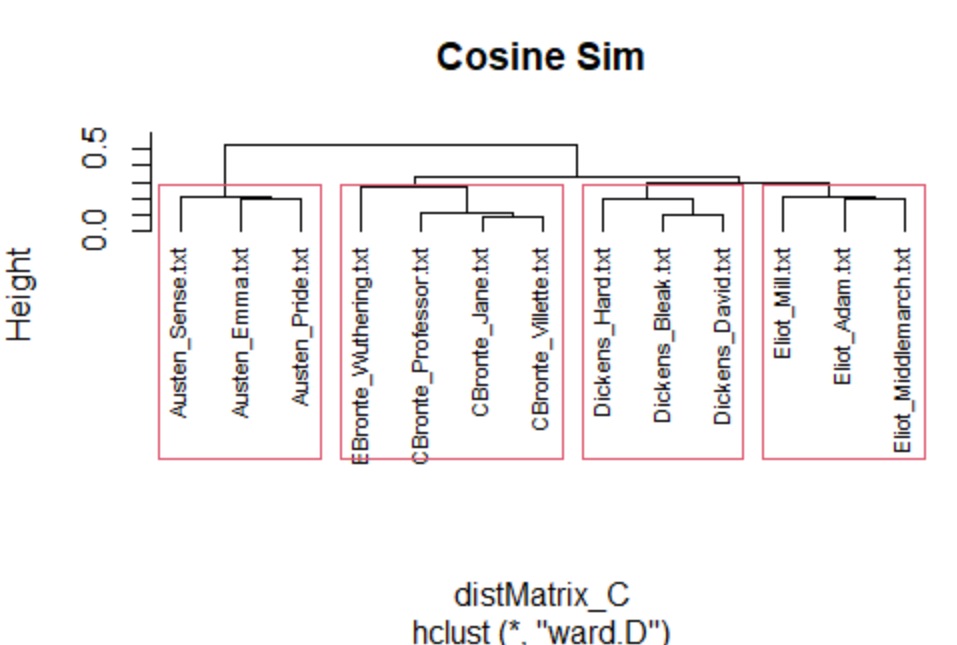
plot(HClust_Ward_CosSim_SmallCorp, cex=.7, hang=-1,main = "Cosine Sim")
rect.hclust(HClust_Ward_CosSim_SmallCorp, k=3)
### OR ### Create your own Cosine Sim Distance Metric function
### This one works much better...........
(My_m <- (as.matrix(scale(t(SmallCorpus_DF_DT)))))
(My_cosine_dist = 1-crossprod(My_m) /(sqrt(colSums(My_m^2)%*%t(colSums(My_m^2)))))
# create dist object
My_cosine_dist <- as.dist(My_cosine_dist) ## Important
HClust_Ward_CosSim_SmallCorp2 <- hclust(My_cosine_dist, method="ward.D")
plot(HClust_Ward_CosSim_SmallCorp2, cex=.7, hang=-30,main = "Cosine Sim")
rect.hclust(HClust_Ward_CosSim_SmallCorp2, k=3)
################## SOOO much more you can do....
# http://www.sthda.com/english/wiki/factoextra-r-package-easy-multivariate-data-analyses-and-elegant-visualization
######################################################
############## FINALLY!! - let's try this on Novels
## Can we cluster authors based on their writing?
######################################
##################################
##
## Novels Corpus
## https://drive.google.com/drive/folders/1xhsk_Dwq4sZ_1q2CtVdSIJWHEZqzMwhG?usp=sharing
##
#######################################
## Next, load in the documents ( from the corpus)
NovelCorpus <- Corpus(DirSource("Novels_Corpus"))
(getTransformations()) ## These work with library tm
(ndocs<-length(NovelCorpus))
## Do some clean-up.............
NovelCorpus <- tm_map(NovelCorpus, content_transformer(tolower))
NovelCorpus <- tm_map(NovelCorpus, removePunctuation)
##-------------------------------------------------------------
## Convert to Document Term Matrix and TERM document matrix
## Each has its own purpose.
## DOCUMENT Term Matrix (Docs are rows)
NovelsCorpus_DTM <- DocumentTermMatrix(NovelCorpus,
control = list(
stopwords = TRUE, ## remove normal stopwords
wordLengths=c(4, 10),
removePunctuation = TRUE,
removeNumbers = TRUE,
tolower=TRUE
#stemming = TRUE,
))
inspect(NovelsCorpus_DTM)
### Create a DF as well................
Novels_DF_DT <- as.data.frame(as.matrix(NovelsCorpus_DTM))
## Create a Novels Matrix
My_novels_m <- (as.matrix(Novels_DF_DT))
nrow(My_novels_m)
## WORD CLOUD
#word.freq <- sort(rowSums(t(My_novels_m)), decreasing = T)
#wordcloud(words = names(word.freq), freq = word.freq*2, min.freq = 2,
# random.order = F)
## COsine Sim
## a * b / (||a|| * ||b||)
CosineSim <- My_novels_m / sqrt(rowSums(My_novels_m * My_novels_m))
CosineSim <- CosineSim %*% t(CosineSim)
#Convert to distance metric
D_Cos_Sim <- as.dist(1-CosineSim)
HClust_Ward_CosSim_SmallCorp2 <- hclust(D_Cos_Sim, method="ward.D2")
plot(HClust_Ward_CosSim_SmallCorp2, cex=.7, hang=-11,main = "Cosine Sim")
rect.hclust(HClust_Ward_CosSim_SmallCorp2, k=4)
###########################################################
##
## This tutorial will not cover csv text files
## But, the following will offer syntax and hints
## in case you have text data in a csv file rather than in a corpus
#######################################################################
#######################################
## In R, there is a PROCESS required
## to convert a csv file into a DTM...
##############################################################
## HERE, "Open" is the name of a dataframe that contains
## open student feedback comments - which is why is it called Open.
## However - the name does not matter. "Open" is a dataframe.
##--------------------------------------------------------------
# head(Open)
# str(Open)
# ## --CONVERT TO TEXT (not factor)
# Open$V1<-as.character(Open$V1) ##V1 stands for variable 1
## --Again- this is example syntax that must be UPDATED for a different
## --dataset.....
# str(Open)
#
# ## Next - and this is crazy hard to find -
# ## In R, when using tm on a csv file
# ## The csv MUST have two columns and the following names: doc_id and text
# ## DO NOT ALTER THESE NAMES!! To add them...use this........
# ## colnames(x) <- c("doc_id", "text")
#
# ## 1) Create a column with the row numbers
# id <- rownames(Open)
# Open <- cbind(doc_id=id, Open)
# ## 2) Make sure the DF has the EXACT column names of doc_id and text....
# colnames(Open) <- c("doc_id", "text")
# ## Check it
# head(Open)
#
# ### CONVERT csv to corpus............................
# OpenCorp <- Corpus(DataframeSource(Open))
# OpenCorp <- tm_map(OpenCorp, tolower) ### DO THIS FIRST before removing specific words!
# OpenCorp <- tm_map(OpenCorp, removeWords, c("also", "that", "this", "with", "anly", "have",
# "class", "classes", "data"))
#
# OpenCorp <- tm_map(OpenCorp, removeWords, stopwords("english"))
# ##OpenCorp <-tm_map(OpenCorp, stemDocument)
# OpenCorp <- tm_map(OpenCorp, lemmatize_strings)
#
# Open_dtm <- DocumentTermMatrix(OpenCorp,
# control = list(
# #stopwords = TRUE,
# wordLengths=c(4, 10),
# removePunctuation = TRUE,
# removeNumbers = TRUE,
# tolower=TRUE,
# remove_separators = TRUE
#
# )
# )
#
# inspect(Open_dtm)
CODE EXAMPLE 2
###
##
### Document Similarity Using Measures
##
## Gates
## ANother good resource:
## https://rstudio-pubs-static.s3.amazonaws.com/66739_c4422a1761bd4ee0b0bb8821d7780e12.html
## http://www.minerazzi.com/tutorials/cosine-similarity-tutorial.pdf
## Book: Text Mining in R
## https://www.tidytextmining.com/
######## Example 1 ----------------------
##
## Whenever you learn something new, always create a very small
## example that you can practice with.

## I have created a small "Corpus" (collections of documents or books)
## They are called, Doc1, Doc2, ..., Doc5.
## The documents are in sentence format.

## The goal is to see how similar the documents are.

## First, we must read in the documents and convert them to
## a format that we can evaluate.

##If you install from the source....
#Sys.setenv(NOAWT=TRUE)
## ONCE: install.packages("wordcloud")
library(wordcloud)
## ONCE: install.packages("tm")
library(tm)
# ONCE: install.packages("Snowball")
## NOTE Snowball is not yet available for R v 3.5.x
## So I cannot use it  - yet...
##library("Snowball")
##set working directory
## ONCE: install.packages("slam")
library(slam)
library(quanteda)
## ONCE: install.packages("quanteda")
## Note - this includes SnowballC
library(SnowballC)
library(arules)
##ONCE: install.packages('proxy')
library(proxy)

setwd("C:\\Users\\profa\\Documents\\RStudioFolder_1\\DrGExamples\\SYR\\IST707\\Week4")
## Next, load in the documents (the corpus)

### !!!!!!!!!
## Make your own corpus with 5 docs
## Make some docs similar to others so that they cluster!
##
## !!!!!!!!!!!!!!!!!!!!!!!!!!!
TheCorpus <- Corpus(DirSource("Corpus"))
##The following will show you that you read in 5 documents
(TheCorpus)

##Next, there are several steps needed to prepare the texts
## You will need to remove punctuation, make everything lowercase
## normalize, remove common and useless words like "and", "the", "or"
## Uselses words are called "Stop Words"
## Don't forget to remove numbers as well.

## The function : getTransformations() will show all the functions
## that process the data - such as removeNumbers, removePunctuation, etc
## run getTransformations() to see this.
## Also note that tolower() will change all case to lowercase.

## The tm_map function allows you to perform the same
## transformations on all of your texts at once
CleanCorpus <- tm_map(TheCorpus, removePunctuation)

## Remove all Stop Words
CleanCorpus <- tm_map(CleanCorpus, removeWords, stopwords("english"))

## You can also remove words that you do not want
MyStopWords <- c("and","like", "very", "can", "I", "also", "lot")
CleanCorpus <- tm_map(CleanCorpus, removeWords, MyStopWords)

## NOTE: If you have many words that you do not want to include
## you can create a file/list
## MyList <- unlist(read.table("PATH TO YOUR STOPWORD FILE", stringsAsFactors=FALSE)
## MyStopWords <- c(MyList)

##Make everything lowercase
CleanCorpus <- tm_map(CleanCorpus, content_transformer(tolower))

## Next, we can apply lemmitization
## In other words, we can combine variations on words such as
## sing, sings, singing, singer, etc.
## NOTE: This will NOT WORK for R version 3.5.x yet - so its
## just for FYI. This required package Snowball which does not yet
## run under the new version of R
#CleanCorpus <- tm_map(CleanCorpus, stemDocument)
#inspect(CleanCorpus)


## Let's see where we are so far...
inspect(CleanCorpus)
## You can use this view/information to add Stopwords and then re-run.
## In other words, I see from inspection that the word "can" is all over
## the place. But it does not mean anything. So I added it to my MyStopWords

## Next, I will write all cleaned docs  - the entire cleaned and prepped corpus
## to a file - in case I want to use it for something else.

(Cdataframe <- data.frame(text=sapply(CleanCorpus, identity),
                        stringsAsFactors=F))
write.csv(Cdataframe, "Corpusoutput2.csv")

## Note: There are several other functions that also clean/prep text data
## stripWhitespace and
## myCorpus <- tm_map(myCorpus, content_transformer(removeURL))

## ------------------------------------------------------------------
## Now, we are ready to move forward.....
##-------------------------------------------------------------------

## View corpus as a document matrix
## TMD stands for Term Document Matrix
(MyTDM <- TermDocumentMatrix(CleanCorpus))
(MyDTM2 <- DocumentTermMatrix(CleanCorpus))
inspect(MyTDM)
inspect(MyDTM2)


## By inspecting this matrix, I see that the words "also" and "lot" is there, but not useful
## I will add these to my MyStopWords and will re-run the above code....
##--------------NOTE
## ABOUT DocumentTermMatrix vs. TermDocumentMatrix - yes these are NOT the same :)
##TermDocument means that the terms are on the vertical axis and the documents are
## along the horizontal axis. DocumentTerm is the reverse

## Before we normalize, we can look at the overall frequencies of words
## This will find words that occur 3 or more times in the entire corpus
(findFreqTerms(MyDTM2, 3))
## Find assocations via correlation
## https://www.rdocumentation.org/packages/tm/versions/0.7-6/topics/findAssocs
findAssocs(MyDTM2, 'coffee', 0.20)
findAssocs(MyDTM2, 'dog', 0.20)
findAssocs(MyDTM2, 'hiking', 0.20)

## VISUALIZE XXXXXXXXXXXXXXXXXXXXXXXXXXXXXXXXXX
## For Document Term Matrix...........
(CleanDF <- as.data.frame(inspect(MyTDM)))
## For Term Doc Matrix...................
(CleanDF2 <- as.data.frame(inspect(MyDTM2)))
(CleanDFScale2 <- scale(CleanDF2))

(CleanDFScale <- scale(CleanDF))
(d_TDM_E <- dist(CleanDFScale,method="euclidean"))
(d_TDM_M <- dist(CleanDFScale,method="minkowski", p=1))
(d_TDM_M3 <- dist(CleanDFScale,method="minkowski", p=3))


library(stylo)
(d_TDM_C <- stylo::dist.cosine(CleanDFScale))


################ Distance Metrics...############
# https://www.rdocumentation.org/packages/stats/versions/3.6.2/topics/dist
###########################################################
(d2_DT_E <- dist(CleanDF2,method="euclidean"))

str(d2_DT_E)
(d2_DT_M2 <- dist(CleanDF2,method="minkowski", p=2))  ##same as Euclidean
(d2_DT_Man <- dist(CleanDFScale2,method="manhattan"))
(d2_DT_M1 <- dist(CleanDFScale2,method="minkowski", p=1)) ## same as Manhattan
(d2_DT_M4 <- dist(CleanDFScale2,method="minkowski", p=4))
(d_DT_C <- stylo::dist.cosine(CleanDFScale2))
#################
## Create hierarchical clustering and dendrograms......................
#https://www.rdocumentation.org/packages/stats/versions/3.6.2/topics/hclust
################

## Term Doc  - to look at words......
fit_TD1 <- hclust(d_TDM_E, method="ward.D2")
plot(fit_TD1)   ## Ward starts with n clusters of size 1 and then combines
## https://en.wikipedia.org/wiki/Ward%27s_method

fit_TD2 <- hclust(d_TDM_M, method="ward.D2")
plot(fit_TD2)

## Doc Term - to look at documents....
fit_DT1 <- hclust(d2_DT_E, method="ward.D")
plot(fit_DT1)

fit_DT2 <- hclust(d2_DT_Man, method="average")
plot(fit_DT2)
## Average distance between two clusters is defined as the mean distance
## between an observation in one cluster and an observation in the other cluster

fit_DT3 <- hclust(d2_DT_M4, method="ward.D2")
plot(fit_DT3)

fit_DT4 <- hclust(d_DT_C, method="ward.D2")
plot(fit_DT4)


## NOw I have a good matrix that allows me to see all the key words of interest
## and their frequency in each document
## HOWEVER - I still need to normalize!
## Even though this example is very small and all docs in this example are about the
## same size, this will not always be the case. If a document has 10,000 words, it
## will easily have a greater frequency of words than a doc with 1000 words.


head(CleanDF2)
str(CleanDF2)

inspect(MyDTM2)
str(MyDTM2)

## Visualize normalized DTM
## The dendrogram:
## Terms higher in the plot appear more frequently within the corpus
## Terms grouped near to each other are more frequently found together
CleanDF_N <- as.data.frame(inspect(MyDTM2))
CleanDFScale_N <- scale(CleanDF_N)
(d <- dist(CleanDFScale_N,method="euclidean"))
fit <- hclust(d, method="ward.D2")
#rect.hclust(fit, k = 4) # cut tree into 4 clusters
plot(fit)

###################################
## frequency Wordcloud
##################################################
library(wordcloud)
library(RColorBrewer)
#install.packages("wordcloud2")
library(wordcloud2)

inspect(MyTDM)  ## term doc (not doc term!)

m <- as.matrix(MyTDM)   ## You can use this or the next for m
(m)
##(t(m))
#m <- as.matrix(CleanDF_N)
# calculate the frequency of words and sort it by frequency
#https://www.rdocumentation.org/packages/wordcloud/versions/2.6/topics/wordcloud
word.freq <- sort(rowSums(m), decreasing = T)
wordcloud(words = names(word.freq), freq = word.freq*2,
          min.freq = 2,
          random.order = F,
          colors=brewer.pal(8, "Dark2"),
          scale=c(3.5,0.05),
          rot.per=0.35)


############### Using wordcloud2 ########################
## Create a special dataframe of words and frequencies
(WordFreqDF<-data.frame(words=names(word.freq), freq=word.freq))
wordcloud2(data=WordFreqDF, size=1.6, color='random-dark')

###############################################
##  kmeans
##
###################################################################

#ClusterM <- t(m) # transpose the matrix to cluster documents
#(ClusterM)
#set.seed(100) # set a fixed random seed
k <- 3 # number of clusters
#(kmeansResult <- kmeans(ClusterM, k))
(kmeansResult_tf_scaled <- kmeans(CleanDFScale_N, k))
(kmeansResult <- kmeans(MyDTM2, k))

#round(kmeansResult$centers, digits = 3) # cluster centers

## See the clusters  - this shows the similar documents
## This does not always work well and can also depend on the
## starting centroids
(kmeansResult$cluster)
plot(kmeansResult$cluster)


#############----------------> Silhouette with fviz
#https://www.rdocumentation.org/packages/factoextra/versions/1.0.7/topics/fviz_nbclust
library("factoextra")

(MyDF<-as.data.frame(as.matrix(MyDTM2), stringsAsFactors=False))
factoextra::fviz_nbclust(MyDF, kmeans, method='silhouette', k.max=5)


inspect(MyDTM2)

(fviz_cluster(kmeansResult, data = MyDTM2,
             ellipse.type = "convex",
             #ellipse.type = "concave",
             palette = "jco",
             axes = c(1, 4), # num axes = num docs (num rows)
             ggtheme = theme_minimal()))
#, color=TRUE, shade=TRUE,
         #labels=2, lines=0)

## Let's try to find similarity using cosine similarity
## Let's look at our matrix

DT1<-MyDTM2
inspect(DT1)

DT_t <- t(MyDTM2) ## for docs
inspect(DT_t)

cosine_dist_mat1 <-
   1 - crossprod_simple_triplet_matrix(DT1)/
   (sqrt(col_sums(DT1^2) %*% t(col_sums(DT1^2))))

(cosine_dist_mat1)

cosine_dist_mat_t <-
  1 - crossprod_simple_triplet_matrix(DT_t)/
  (sqrt(col_sums(DT_t^2) %*% t(col_sums(DT_t^2))))

(cosine_dist_mat_t)

#heatmap https://www.rdocumentation.org/packages/stats/versions/3.5.0/topics/heatmap
## Simiarity between words
png(file="HeatmapCosSimExample.png", width=1600, height=1600)
heatmap(cosine_dist_mat1, cexRow=3, cexCol = 3)
dev.off()

#pdf(file="HeatmapCosSimExample.pdf")
(heatmap(cosine_dist_mat_t))

## Simiarity between words

heatmap(t(cosine_dist_mat1),cexRow=.5, cexCol = .5 )

##############----------------------------------------
#install.packages('heatmaply')
#install.packages('yaml')
library(heatmaply)
library(htmlwidgets)
library(yaml)
mat<-t(cosine_dist_mat1)
p <- heatmaply(mat,
               #dendrogram = "row",
               xlab = "", ylab = "",
               main = "",
               scale = "column",
               margins = c(60,100,40,20),
               grid_color = "white",
               grid_width = 0.00001,
               titleX = FALSE,
               hide_colorbar = TRUE,
               branches_lwd = 0.1,
               label_names = c("A", "B", "C"),
               fontsize_row = 5, fontsize_col = 5,
               labCol = colnames(mat),
               labRow = rownames(mat),
               heatmap_layers = theme(axis.line=element_blank())
            )


# save the widget
#
saveWidget(p, file= "heatmaplyExample.html")

## For the Docs
## You can use any of the distance metrics...
(mat<-as.matrix(d2_DT_E ))

p2 <- heatmaply(mat,
               #dendrogram = "row",
               xlab = "", ylab = "",
               main = "",
               scale = "column",
               margins = c(60,100,40,20),
               grid_color = "white",
               grid_width = 0.00001,
               titleX = FALSE,
               hide_colorbar = TRUE,
               branches_lwd = 0.2,
               label_names = c("A", "B", "C"),
               fontsize_row = 5, fontsize_col = 5,
               labCol = colnames(mat),
               labRow = rownames(mat),
               heatmap_layers = theme(axis.line=element_blank())
              )


# save the widget
#
saveWidget(p2, file= "heatmaplyExample2.html")


#################################################################
## This is a small example of cosine similarity so you can see how it works
## I will comment it out...
######  m3 <- matrix(1:9, nrow = 3, ncol = 3)
######   (m3)
######   ((crossprod(m3))/(  sqrt(col_sums(m3^2) %*% t(col_sums(m3^2))   )))
####################################################################################

##########################################################3
##
##   Silhouette and Elbow - choosing k
##
#########################################################################
#https://www.r-bloggers.com/2019/01/10-tips-for-choosing-the-optimal-number-of-clusters/
# The Elbow Curve method is helpful because it shows how
# increasing the number of the clusters contribute
# separating the clusters in a meaningful way,
# not in a marginal way.
# The bend indicates that additional clusters beyond
# the third have little value.
#####################################################################


fviz_nbclust(
  as.matrix(MyDTM2),
  kmeans,
  k.max = 5,
  method = "wss",
  diss = get_dist(as.matrix(MyDTM2), method = "spearman")
)

fviz_nbclust(
  as.matrix(MyDTM2),
  kmeans,
  k.max = 5,
  method = "wss",
  diss = get_dist(as.matrix(MyDTM2), method = "euclidean")
)


##
## https://bradleyboehmke.github.io/HOML/kmeans.html#determine-k
#install.packages('cluster')
library(cluster)
#(dist_mat<-as.matrix(d2_DT_E))
## Silhouette........................
fviz_nbclust(CleanDF2, method = "silhouette", FUN = hcut, k.max = 4)


#######################------------>

##############################################
##  Other Forms of CLustering.........
##
#########################################################
## HIERARCHICAL

# ----
library(dplyr)       # for data manipulation
library(ggplot2)     # for data visualization

# ---
#install.packages("cluster")
library(cluster)     # for general clustering algorithms
library(factoextra)  # for visualizing cluster results

## DATA
###https://drive.google.com/file/d/1x3PVxYAmx7CdxB6N5bF-30Z0tq9guvja/view?usp=sharing

filename="C:/Users/profa/Documents/RStudioFolder_1/DrGExamples/ANLY503/HeartRiskData_Outliers.csv"
HeartDF2<-read.csv(filename)
head(HeartDF2)
str(HeartDF2)
summary(HeartDF2)

HeartDF2$StressLevel<-as.ordered(HeartDF2$StressLevel)
HeartDF2$Weight<-as.numeric(HeartDF2$Weight)
HeartDF2$Height<-as.numeric(HeartDF2$Height)
str(HeartDF2)
head(HeartDF2)

## !!!!!!!!!!!!!!!!!
## You CANNOT use distance metrics on non-numeric data
## Before we can proceed - we need to REMOVE
## all non-numeric columns

HeartDF2_num <- HeartDF2[,c(3,5,6)]
head(HeartDF2_num)


# Dissimilarity matrix with Euclidean
## dist in R
##  "euclidean", "maximum", "manhattan",
## "canberra", "binary" or "minkowski" with p
(dE <- dist(HeartDF2_num, method = "euclidean"))
(dM <- dist(HeartDF2_num, method = "manhattan"))
(dMp2 <- dist(HeartDF2_num, method = "minkowski", p=2))

# Hierarchical clustering using Complete Linkage
(hc_C <- hclust(dM, method = "complete" ))
plot(hc_C)
## RE:
#https://www.rdocumentation.org/packages/stats/versions/3.6.2/topics/hclust
# Hierarchical clustering with Ward
# ward.D2" = Ward's minimum variance method -
# however dissimilarities are **squared before clustering.
# "single" = Nearest neighbours method.
# "complete" = distance between two clusters is defined
# as the maximum distance between an observation in one.
hc_D <- hclust(dE, method = "ward.D" )
plot(hc_D)
hc_D2 <- hclust(dMp2, method = "ward.D2" )
plot(hc_D2)

######## Have a look ..........................
plot(hc_D2)
plot(hc_D)
plot(hc_C)


##################################################
##
## Which methods to use??
##
## Method with stronger clustering structures??
######################################################
library(purrr)
#install.packages("cluster")

library(cluster)

methods <- c( "average", "single", "complete", "ward")
names(methods) <- c( "average", "single", "complete", "ward")


# function to compute coefficient
MethodMeasures <- function(x) {
  cluster::agnes(HeartDF2_num, method = x)$ac
}

# The agnes() function will get the agglomerative coefficient (AC),
# which measures the amount of clustering structure found.
# Get agglomerative coefficient for each linkage method
(purrr::map_dbl(methods, MethodMeasures))
#average    single  complete      ward
#0.9629655 0.9642673 0.9623190 0.9645178
# We can see that single is best in this case


############################################
## More on Determining optimal clusters
#######################################################
library("factoextra")
# Look at optimal cluster numbers using silh, elbow, gap
(WSS <- fviz_nbclust(HeartDF2_num, FUN = hcut, method = "wss",
                   k.max = 5) +
  ggtitle("WSS:Elbow"))
SIL <- fviz_nbclust(HeartDF2_num, FUN = hcut, method = "silhouette",
                   k.max = 5) +
  ggtitle("Silhouette")
GAP <- fviz_nbclust(HeartDF2_num, FUN = hcut, method = "gap_stat",
                   k.max = 5) +
  ggtitle("Gap Stat")

# Display plots side by side
gridExtra::grid.arrange(WSS, SIL, GAP, nrow = 1)

############ and ...............
library(factoextra)
file2<-"C:/Users/profa/Documents/RStudioFolder_1/DrGExamples/ANLY503/HeartRisk.csv"
#data
# https://drive.google.com/file/d/1pt-ouIQXH-SQzUMSqbl6Z6UWZrY3i4qu/view?usp=sharing
HeartDF_no_outliers<-read.csv(file2)
head(HeartDF_no_outliers)
## Remove non-numbers
HeartDF_no_outliers_num<-HeartDF_no_outliers[,c(3,5,6)]
head(HeartDF_no_outliers_num)

## Use a distance metric
Dist_E<-dist(HeartDF_no_outliers_num, method = "euclidean" )
fviz_dist(Dist_E)

## If we change the row numbers to labels - we can SEE the clusters...
head(HeartDF_no_outliers)
## Save the first column of labels as names....
(names<-HeartDF_no_outliers[,c(1)])
str(names)
(names<-as.character(names))
## Here is an issue - row names need to be unique.
## So - we need to append numbers to each to make them unique...
(names<-make.unique(names, sep = ""))
## set the row names of the HeartDF_no_outliers_num as these label names...
## What are they now?
row.names(HeartDF_no_outliers_num)
## Change them-->
(.rowNamesDF(HeartDF_no_outliers_num, make.names=FALSE) <- names)
##check
row.names(HeartDF_no_outliers_num)

## OK!! Fun tricks! Now - let's cluster again....
Dist_E<-dist(HeartDF_no_outliers_num, method = "euclidean" )
fviz_dist(Dist_E)

## Better!
## NOw we can understand the clusters
## Normally - this is NOT possible
## because many datasets do not have labels

###############################################
##
##  Density Based Clustering
##  -  BDSCAN -
##
####################################################
## Example 1: Trying to use k means for data that
## is NOT in concave clusters...this WILL NOT work....
##----------------------------
library(factoextra)
data("multishapes")
df <- multishapes[, 1:2]
set.seed(123)
km.res <- kmeans(df, 5, nstart = 25)
fviz_cluster(km.res, df, frame = FALSE, geom = "point")

## Example 2: Using Density Clustering........
#install.packages("fpc")
#install.packages("dbscan")
library(fpc)
library(dbscan)

data("multishapes", package = "factoextra")
df <- multishapes[, 1:2]
db <- fpc::dbscan(df, eps = 0.15, MinPts = 5)
# Plot DBSCAN results
plot(db, df, main = "DBSCAN", frame = FALSE)

## REF: http://www.sthda.com/english/wiki/wiki.php?id_contents=7940
CODE EXAMPLE 3:
The following code will show many clustering examples and visualization options in R.
This data works on a corpus of novels, but can be updated to work on other text or record
data.
#########################################################
##
##          Tutorial: Text Mining and NLP
## Note to Ami: Clustering and Distance with Novels.R
## ...707\Week4
##           Topics:
##             - Tokenization
##             - Vectorization
##             - Normalization
##             - classification/Clustering
##             - Visualization
##
##     THE DATA CORPUS IS HERE:
##  https://drive.google.com/drive/folders/1J_8BDiOttPvEYW4-JxrReKGP1wN40ccy?usp=sharing
#########################################################
## Gates
#########################################################


library(tm)
#install.packages("tm")
library(stringr)
library(wordcloud)
# ONCE: install.packages("Snowball")
## NOTE Snowball is not yet available for R v 3.5.x
## So I cannot use it  - yet...
##library("Snowball")
##set working directory
## ONCE: install.packages("slam")
library(slam)
library(quanteda)
## ONCE: install.packages("quanteda")
## Note - this includes SnowballC
library(SnowballC)
library(arules)
##ONCE: install.packages('proxy')
library(proxy)
library(cluster)
library(stringi)
library(proxy)
library(Matrix)
library(tidytext) # convert DTM to DF
library(plyr) ## for adply
library(ggplot2)
library(factoextra) # for fviz
library(mclust) # for Mclust EM clustering
library(textstem)  ## Needed for lemmatize_strings

library(amap)  ## for Kmeans
library(networkD3)

######### LINK TO NOVELS CORPUS
##
## https://drive.google.com/drive/folders/1CZ75yZ9saow5o8sB1RsFGx6N4T8Xe8hL?usp=sharing
#################################################

####### USE YOUR OWN PATH ############
setwd("C:/Users/profa/Documents/RStudioFolder_1/DrGExamples")

## Next, load in the documents (the corpus)
NovelsCorpus <- Corpus(DirSource("Novels_Corpus"))
(getTransformations()) ## These work with library tm
(ndocs<-length(NovelsCorpus))

NovelsCorpus <- tm_map(NovelsCorpus, content_transformer(tolower))
NovelsCorpus <- tm_map(NovelsCorpus, removePunctuation)
## Remove all Stop Words
#NovelsCorpus <- tm_map(NovelsCorpus, removeWords, stopwords("english"))

## You can also remove words that you do not want
#MyStopWords <- c("and","like", "very", "can", "I", "also", "lot")
#NovelsCorpus <- tm_map(NovelsCorpus, removeWords, MyStopWords)
NovelsCorpus <- tm_map(NovelsCorpus, lemmatize_strings)

##The following will show you that you read in all the documents
(summary(NovelsCorpus))  ## This will list the docs in the corpus
(meta(NovelsCorpus[[1]])) ## meta data are data hidden within a doc - like id
(meta(NovelsCorpus[[1]],5))

###################################################################
#######       Change the COrpus into a DTM, a DF, and  Matrix
#######
####################################################################
## There are OPTIONS. This is NOT what you should do - but rather
## things you can do, consider, and learn more about.

# You can ignore extremely rare words i.e. terms that appear in less
# then 1% of the documents. The following is an EXAMPLE not a set method
##(minTermFreq <- ndocs * 0.01) ## Because we only have 13 docs - this will not matter
# You can ignore overly common words i.e. terms that appear in more than
## 50% of the documents
##(maxTermFreq <- ndocs * .50)

## You can create your own Stopwords
## A Wordcloud is good to determine
## if there are odd words you want to remove
#(STOPS <- c("aaron","maggi", "maggie", "philip", "tom", "glegg", "deane", "stephen","tulliver"))

Novels_dtm <- DocumentTermMatrix(NovelsCorpus,
                         control = list(
                           stopwords = TRUE, ## remove normal stopwords
                           wordLengths=c(4, 10), ## get rid of words of len 3 or smaller or larger than 15
                           removePunctuation = TRUE,
                           removeNumbers = TRUE,
                           tolower=TRUE,
                           #stemming = TRUE,
                           remove_separators = TRUE
                           #stopwords = MyStopwords,

                           #removeWords(MyStopwords),
                           #bounds = list(global = c(minTermFreq, maxTermFreq))
                         ))
########################################################
################### Have a look #######################
################## and create formats #################
########################################################
#(inspect(Novels_dtm))  ## This takes a look at a subset - a peak
DTM_mat <- as.matrix(Novels_dtm)
DTM_mat[1:13,1:10]

#########################################################
######### OK - Pause - now the data is vectorized ######
## Its current formats are:
## (1) Novels_dtm is a DocumentTermMatrix R object
## (2) DTM_mat is a matrix
#########################################################

#Novels_dtm <- weightTfIdf(Novels_dtm, normalize = TRUE)
#Novels_dtm <- weightTfIdf(Novels_dtm, normalize = FALSE)

## Look at word freuqncies out of interest
(WordFreq <- colSums(as.matrix(Novels_dtm)))

(head(WordFreq))
(length(WordFreq))
ord <- order(WordFreq)
(WordFreq[head(ord)])
(WordFreq[tail(ord)])
## Row Sums
(Row_Sum_Per_doc <- rowSums((as.matrix(Novels_dtm))))

## I want to divide each element in each row by the sum of the elements
## in that row. I will test this on a small matrix first to make
## sure that it is doing what I want. YOU should always test ideas
## on small cases.
#############################################################
########### Creating and testing a small function ###########
#############################################################
## Create a small pretend matrix
## Using 1 in apply does rows, using a 2 does columns
(mymat = matrix(1:12,3,4))
freqs2 <- apply(mymat, 1, function(i) i/sum(i))  ## this normalizes
## Oddly, this re-organizes the matrix - so I need to transpose back
(t(freqs2))
##  !!!!!!!!!!!!!!!!!
## OK - so this works.
## !!!!!!!!!!!!!!!!!
##  ** Now I can use this to control the normalization of
## my matrix...
#############################################################

## Copy of a matrix format of the data
Novels_M <- as.matrix(Novels_dtm)
(Novels_M[1:13,1:5])

## Normalized Matrix of the data
Novels_M_N1 <- apply(Novels_M, 1, function(i) round(i/sum(i),3))
(Novels_M_N1[1:13,1:5])
## NOTICE: Applying this function flips the data...see above.
## So, we need to TRANSPOSE IT (flip it back)  The "t" means transpose
Novels_Matrix_Norm <- t(Novels_M_N1)
(Novels_Matrix_Norm[1:13,1:10])

############## Always look at what you have created ##################
## Have a look at the original and the norm to make sure
(Novels_M[1:13,1:10])
(Novels_Matrix_Norm[1:13,1:10])

######################### NOTE #####################################
## WHen you make calculations - always check your work....
## Sometimes it is better to normalize your own matrix so that
## YOU have control over the normalization. For example
## scale used diectly may not work - why?

##################################################################
###############   Convert to dataframe     #######################
##################################################################

## It is important to be able to convert between format.
## Different models require or use different formats.
## First - you can convert a DTM object into a DF...
(inspect(Novels_dtm))
Novels_DF <- as.data.frame(as.matrix(Novels_dtm))

#str(Novels_DF)
(Novels_DF$aunt)   ## There are 13 numbers... why? Because there are 13 documents.
Novels_DF[1:3, 1:10]
(nrow(Novels_DF))  ## Each row is a novel
## Fox DF format
ncol(Novels_DF)
######### Next - you can convert a matrix (or normalized matrix) to a DF
Novels_DF_From_Matrix_N<-as.data.frame(Novels_Matrix_Norm)

#######################################################################
#############   Making Word Clouds ####################################
#######################################################################
## This requires a matrix - I will use Novels_M from above.
## It is NOT mornalized as I want the frequency counts!
## Let's look at the matrix first
(Novels_M[c(1:13),c(3850:3900)])
wordcloud(colnames(Novels_M), Novels_M[13, ], max.words = 100)

############### Look at most frequent words by sorting ###############
(head(sort(Novels_M[13,], decreasing = TRUE), n=20))

#######################################################################
##############        Distance Measures          ######################
#######################################################################
## Each row of data is a novel in this case
## The data in each row are the number of time that each word occurs
## The words are the columns
## So, distances can be measured between each pair of rows (or each novel)
## We can determine which novels (rows of numeric word frequencies) are "closer"
########################################################################
## 1) I need a matrix format
## 2) I will use the matrix above that I created and normalized:
##    Novels_Matrix_Norm
## Let's look at it
(Novels_Matrix_Norm[c(1:6),c(3850:3900)])
## 3) For fun, let's also do this for a non-normalized matrix
##    I will use Novels_M from above
## Let's look at it
(Novels_M[c(1:6),c(3850:3900)])

## I am going to make copies here.
m  <- Novels_M
m_norm <-Novels_Matrix_Norm
(str(m_norm))

###############################################################################
################# Build distance MEASURES using the dist function #############
###############################################################################
## Make sure these distance matrices make sense.
distMatrix_E <- dist(m, method="euclidean")
print(distMatrix_E)

distMatrix_C <- dist(m, method="cosine")
print("cos sim matrix is :\n")
print(distMatrix_C) ##small number is less distant

print("L2 matrix is :\n")
print(distMatrix_E)

distMatrix_C_norm <- dist(m_norm, method="cosine")
print("The norm cos sim matrix is :\n")
print(distMatrix_C_norm)

(distMatrix_Min_2 <- dist(m,method="minkowski", p=2))
###########################################################################

############# Clustering #############################
## Hierarchical

## Euclidean
groups_E <- hclust(distMatrix_E,method="ward.D")
plot(groups_E, cex=0.9, hang=-1, main = "Euclidean")
rect.hclust(groups_E, k=4)

## From the NetworkD3 library
#https://cran.r-project.org/web/packages/networkD3/networkD3.pdf
radialNetwork(as.radialNetwork(groups_E))

## Cosine Similarity
groups_C <- hclust(distMatrix_C,method="ward.D")
plot(groups_C, cex=.7, hang=-30,main = "Cosine Sim")
rect.hclust(groups_C, k=4)

radialNetwork(as.radialNetwork(groups_C))
dendroNetwork(groups_C)


## Cosine Similarity for Normalized Matrix
groups_C_n <- hclust(distMatrix_C_norm,method="ward.D")
plot(groups_C_n, cex=0.9, hang=-1,main = "Cosine Sim and Normalized")
rect.hclust(groups_C_n, k=4)

radialNetwork(as.radialNetwork(groups_C_n))

### NOTES: Cosine Sim works the best. Norm and not norm is about
## the same because the size of the novels are not sig diff.

####################   k means clustering -----------------------------
## Remember that kmeans uses a matrix of ONLY NUMBERS
## We have this so we are OK.
## Manhattan gives the best vis results!
# https://cran.r-project.org/web/packages/factoextra/factoextra.pdf
## Python Distance Metrics...
## https://towardsdatascience.com/calculate-similarity-the-most-relevant-metrics-in-a-nutshell-9a43564f533e
############################################

#distance matrix is from above....
fviz_dist(distMatrix_C_norm, gradient = list(low = "#00AFBB",
                                     mid = "white", high = "#FC4E07"))+
  ggtitle("Cosine Sim  - normalized- Based Distance Map")


#-

distance0 <- get_dist(m_norm,method = "euclidean")
fviz_dist(distance0, gradient = list(low = "#00AFBB",
                                     mid = "white", high = "#FC4E07"))+
  ggtitle("Euclidean Based Distance Map")


#-
distance1 <- get_dist(m_norm,method = "manhattan")
fviz_dist(distance1, gradient = list(low = "#00AFBB",
                                     mid = "white", high = "#FC4E07"))+
  ggtitle("Manhattan Based Distance Map")


#-
distance2 <- get_dist(m_norm,method = "pearson")
fviz_dist(distance2, gradient = list(low = "#00AFBB",
                                     mid = "white", high = "#FC4E07"))+
  ggtitle("Pearson Based Distance Map")


#-
distance3 <- get_dist(m_norm,method = "canberra")
fviz_dist(distance3, gradient = list(low = "#00AFBB",
                                     mid = "white", high = "#FC4E07"))+
  ggtitle("Canberra Based Distance Map")


#-
distance4 <- get_dist(m_norm,method = "spearman")
fviz_dist(distance4, gradient = list(low = "#00AFBB",
                                     mid = "white", high = "#FC4E07"))+
  ggtitle("Spearman Based Distance Map")


###########################################################
###                 k means  pART 1
#####################################################################
# https://bradleyboehmke.github.io/HOML/kmeans.html
## First - have a look at a small fraction of m
## Recall that m is our novels text DF as a matrix
m[1:10,1:10]
## Next, our current matrix does NOT have the columns as the docs
## so we need to transpose it first....
## Run the following twice...
(nrow(m))   ## m has 13 rows because there are 13 novels in the corpus
(ncol(m))   ## Here we have 31,004 columns: the number of words
#str(m_norm)
## k means
## # Use k-means model with 4 centers and 4 random starts
kmeansFIT_1 <- kmeans(m,centers=4, nstart=4)
(kmeansFIT_1$centers)
#print("Kmeans details:")
summary(kmeansFIT_1)
(kmeansFIT_1$cluster)
kmeansFIT_1$centers[,1]

###############NOTE
## One issue here is that kmeans does not
## allow us to use cosine sim
## This is creating results that are not as good.
####################

### This is a cluster vis
fviz_cluster(kmeansFIT_1, m)
## --------------------------------------------
#########################################################


####################################################
##
##             kmeans part 2
##
########################################################
## x is a numeric matrix of data
## centers: number of clusters or a set of initial cluster centers.
#  nstart: If centers is a number, how many random sets should be chosen
## distance measure:  "euclidean", "maximum", "manhattan", "canberra", "binary",
## "pearson" , "abspearson" , "abscorrelation", "correlation", "spearman" or "kendall"
#install.packages("amap")
library("amap")   ## contains Kmeans

## Check the data...
m[1:10,1:10]
str(m)

## Run Kmeans...
My_Kmeans1<-Kmeans(m, centers=4,method = "euclidean")
#, iter.max = 10, nstart = 1)
fviz_cluster(My_Kmeans1, m, main="Euclidean")

My_Kmeans2<-Kmeans(m, centers=4,method = "spearman")
fviz_cluster(My_Kmeans2, m, main="Spearman")

My_Kmeans3<-Kmeans(m, centers=4,method = "manhattan")
fviz_cluster(My_Kmeans3, m, main="Manhattan")

## akmeans packages........
##d.metric=2 is cosine sim   (1 is euclidean)
## RE: https://cran.r-project.org/web/packages/akmeans/akmeans.pdf
#install.packages("akmeans")
library("akmeans")
My_Adaptive_kmeans_withCosSim<-akmeans(m,d.metric=2,ths3=0.8,mode=3)
My_Adaptive_kmeans_withCosSim$cluster
plot(My_Adaptive_kmeans_withCosSim$cluster)


########### Frequencies and Associations ###################

## FInd frequenct words...
(findFreqTerms(Novels_dtm, 2500))
## Find assocations with aselected conf
(findAssocs(Novels_dtm, 'aunt', 0.95))

############################# Elbow Methods ###################

fviz_nbclust(
  as.matrix(Novels_dtm),
  kmeans,
  k.max = 10,
  method = "wss",
  diss = get_dist(as.matrix(Novels_dtm), method = "manhattan")
)

fviz_nbclust(
  as.matrix(Novels_dtm),
  kmeans,
  k.max = 9,
  method = "wss",
  diss = get_dist(as.matrix(Novels_dtm), method = "spearman")
)

## Silhouette........................
fviz_nbclust(Novels_DF, method = "silhouette",
             FUN = hcut, k.max = 9)