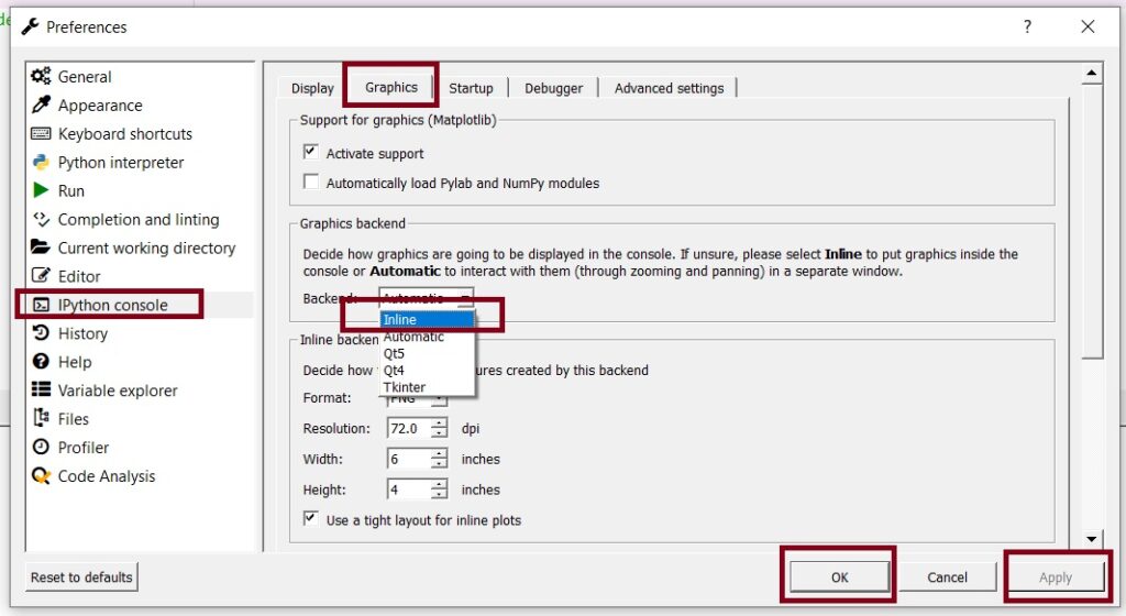
The following code will apply gradient descent to simple linear regression. To properly see the visual element, you will need to view your plots inline (I use the Spyder IDE). To use my code, it is best to understand each line, make updates (such as paths), etc. If you simply copy/paste, it is not likely to run.
HOW TO Update the Plots to Show Inline in the Spyder IDE.

The Code:
# -*- coding: utf-8 -*-
"""
Created on Mon Dec  9 20:08:00 2024

@author: profa
"""

import numpy as np
import pandas as pd
import matplotlib.pyplot as plt
import time

plt.rcParams["figure.figsize"] = (12, 9)

# Place your path here !!
datafile="C:/Users/profa/Desktop/Datasets/ExamScore_HoursStudy_DataSet.csv"


## Here is the small dataset I am using for this example
# HoursOfStudy(x)	ExamScore(y)
# 1	     60
# 2	     72
# 6	     95
# 4.1	     83
# 5	     91
# 1.2	     69
# 7.3	     99
# 4.9	     88


InputData=pd.read_csv(datafile)
print(InputData)
X=InputData.iloc[:,0]
y=InputData.iloc[:,1]

print(X)
print(type(X))
print(y)

plt.scatter(X, y)
# Add gridlines
plt.grid(True)
# Set the title
plt.title("Exam Score (y) and Hours Of Study (x)")
# Set the x and y labels
plt.xlabel("Hours of Study")
plt.ylabel("Exam Score")
plt.show()

## Set up initial weights and biases
m = 0
b = 0

## Learning rate
LR = .1
epochs=70

## What is our Loss function?
## How do we calculate the error
## between y_hat and y (what
## we predict and what is true?)
##
## MSE = 1/n SUM (y_hat - y)^2

epochslist=[]
AllErrors=[]
TotalE = 0
n = len(X)

for i in range(epochs):
    print("Epoch \n", i)
    epochslist.append(i)
    y_hat = m*X + b
    #print("y_hat is\n", y_hat)
    #print("y is\n", y)
    #Error=(1/n) * np.sqrt((y_hat - y)**2)

    ## This is the sum of all the squared errors
    Error=sum((y_hat - y)**2)## MSE

    print(" Error is\n", Error)
    AllErrors.append(Error)

    ## This is how the Loss Function changes with respect to w
    ## The Loss function L we will use is the Mean Squared Error (MSE)
    ## L = 1/n (y_hat - y)^2
    ## Recall that y_hat = mx + b
    dL_dm = 2/n*(X * (y_hat - y ))
    #print(dL_dm)
    dL_db = 2/n*(y_hat - y )

    ## Use the derivatives and the learning rate LR to update m and b
    m = m - ( LR * dL_dm )
    b = b - (LR * dL_db)

    plt.scatter(X,y)
    plt.plot([min(X), max(X)], [min(y_hat), max(y_hat)], color="green")
    plt.show()
    time.sleep(.1)

## End of for loop for epochs

plt.scatter(epochslist, AllErrors)
plt.show()