Advanced Multiple Linear Regression – Quantitative and Categorical Independent Variables – Parameter Interpretation and Related Details.
Author: Ami Gates
Overview
This tutorial will review and discuss the multiple linear regression parametric model for which the independent variables are both quantitative and categorical.
Our focus will be on data preparation, parameter interpretation, R and Python examples, challenges and measures, and discussion.
Review and Common Terminology
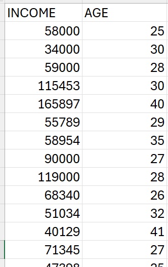
Simple Linear Regression: Recall that simple linear regression estimates a dependent variable using one independent variable.
For example, using the dataset to the right, we can create a model that seeks to predict or estimate “INCOME” using “AGE”.
y = b + w1x1
- “y” is often used to represent the dependent variable. The dependent variable is what we are trying to predict – to model. It is also often called the “target”, “prediction”, or “response variable”. Given our example here, our dependent variable is “INCOME”.
- x1 in this example represents the independent variable. This is also often called the “predictor variable”, or the “regressor”. In this example, our independent variable is “AGE”.
- w1 in this example is a parameter in this parametric linear model. It “weights” the effect that our independent variable, x1, has on our dependent variable, y. This is also often called the “coefficient”, “regression coefficient”, or “beta coefficient (for standardized quantitative independent variables)”.
- b is also a parameter in this linear model. It is often referred to as the bias or intercept.
Our goal here is to use the data that we have to estimate the model parameters (b and w1) so that we can then use the model (and AGE) to estimate INCOME.
It is also important to note that the “letters” used in the model do not matter. For example, the following formula is also for simple linear regression. Here, the y^ (called y hat) is the dependent variable, beta 1 is the weight or coefficient of the independent variable, and beta 0 is the bias.

Multiple Linear Regression (Quantitative only)
Multiple linear regression (MLR) is an extension of SLR that allows many weighted independent variables to estimate or model the dependent variable.
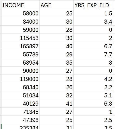
The dataset to the left is very similar to the dataset above. However, in this case, we will use both AGE (x1) and YRS_EXP_FLD (x2) to model and predict the INCOME (y).
Our multiple linear equation could then take the following form.:
y = b + w1x1 + w2x2
Here, we have three parameters: b, w1, and w2.
In this case, both w1 and w2 are the coefficients and b is the bias term.
Specifically, w1 “weights” or controls the effect that the independent variable x1 (AGE) has in predicting y(INCOME). Similarly, w2 “weights” or controls the effect that the independent variable x2(YRS_EXP_FLD) has in predicting y (INCOME).
We can also represent MLR using any letters we wish.

Multiple Linear Regression Using Both Quantitative and Categorical Independent Variables
Part 1: Preparing the Data
So far, our Linear Regression Models have involved only quantitative variables. However, this may not always be the case. Often, the data we have contains both quantitative and categorical variables.
The dataset to the right further extends our independent variables. Here, we will use AGE, YRS_EXP_FLD, and EDU_ to build a linear model with the goal of predicting/estimating INCOME.
Thinking Question: Can we simply create a model like this…
y = b + w1x1 + w2x2 + w3x3, where x1 is AGE, x2 is YRS_EXP_FLD, and x3 is EDU_?
The answer is no. The independent variable, “EDU_” is not quantitative (and is actually categorical). We cannot treat it like a number – for example, we cannot multiply a coefficient value (which is numeric) times a category such as BS.
To use categorical variables as independent variables in linear regression, we will need first to encode the categories.
Is it OK to just encode AA as “0”, BS as “1”, MS as”2″, and PhD as “3”? (Why not?)

Using Categorical Variables in Multiple Linear Regression: Preparing the Data with One-Hot Encoding (Dummy Variables)
One Hot Encoding is an encoding method that can be used to represent categorical variables while avoiding issues such as imposed order or implied value. This is also often referred to in this case as creating dummy variables/indicator variables, where each dummy indicates the presence or absence of a category (in our case AA, BS, MS, or PhD).
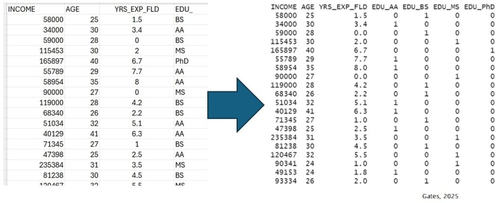
One Hot Encoding Example: The categorical independent variable in our dataset (below) is called “EDU_“. The EDU_ variable can be one of four possible categories in this dataset: “AA”, “BS”, “MS”, or “PhD”.
Because there are four possible categories, we can encode them by creating four dummy variables where only one of the new dummy variables will be a “1” (for a given data row) and all others will be “0”. For example, int he dataset below you can see that the first row has an EDU_ value of “BS“. Therefore, the dummy for BS will be 1 and all other dummies in that row will be 0. The image below illustrates this for each row.
Another way to think about this is a that we are using a vector of size 4 where all the values are 0 except for the one that is ON or HOT, and corresponds to a specific categorical value.
Example: [0 1 0 0] can one-hot encode the BS category from the EDU_ variable.
The image below illustrates the one-hot encoding and transformation for the categorical EDU_ variable (left) into four dummy variables (EDU_AA, EDU_BS, EDU_MS, and EDU_PhD) on the right. Notice that because the first row of data on the left has the value of BS for the variable EDU_ we see that on the right it has been encoded as [0 1 0 0] where the “1” is under the new dummy variable for EDU_BS.
Multicollinearity – Drop First (and Options) – and the Dummy Variable Trap (DVT)
Perfect multicollinearity – which will occur when using all dummy columns (in the presence of the intercept that is not set to 0) can very negatively affect the model and related interpretation.
A common definition is: (Paraphrased – reference) When you include all dummy variables for a categorical variable without dropping one, and also have a non-zero intercept in your regression model, it creates a situation called the “dummy variable trap,” which leads to perfect multicollinearity because one variable (via the sum of all dummy variables) is perfectly linearly dependent on the others, making it impossible to isolate the unique effect of each dummy variable on the dependent variable.
If we remove/drop one of the dummy columns that we created to represent our one categorical variable (EDU_), then we no longer have perfect multicollinearity.
For example, let’s remove the EDU_BS column. (We will talk more about which column to remove in a second). Then, suppose we know that EDU_AA is 1, EDU_BS is 0. Do we know absolutely know the value of EDU_MS? The answer is no. It could be 0 or 1.
Therefore, we no longer have the issue. This method of dropping one of the columns created from one-hot encoding the a categorical independent variable is often called “Drop First” or “dropping the reference/baseline category“.
Drop First is a method commonly used to manage the issue of perfect multicollinearity or the Dummy Variable Trap (DVT).
The general method is to remove (or drop) one of the columns from the dummies created to represent the categorical variable. (If there are many categorical variables – each with dummies – then one would drop a dummy from each.)
The implication of “drop first” is that we arbitrarily remove the first dummy column. Since R and Python alphabetize variables after processing (though you can control this) it is most often the case that the drop is made based on whichever dummy appears first. For example, R will auto-drop the first dummy unless you code it to do otherwise. (The code I am providing below for R and Python is written to avoid the first drop method).
Dropping the Right Dummy – Rather than the first Dummy
While the default is “first”, it is strongly suggested that you think about how you plan to compare and understand the results of the coefficients of the MLR Model.
Then choose to drop the right dummy for the goals of the hypothesis and interpretation.
Let’s better understand what dropping a dummy does, and how this is also connected to the presence and role of the intercept.
- The intercept term in regression model represents a baseline or reference value when all the independent variables are zero. This also explains why we must drop one of the dummy variables – otherwise, we could not have a situation where all independent variables are 0.
- The intercept captures the baseline or reference value represented by the dummy that was dropped. This is critical in the way we interpret the coefficients and model results.
When we drop a dummy variable, it becomes a baseline or reference point for interpreting the regression model results. For this reason, we want to drop the right dummy.
For example, in our dataset, we have four dummies because our categorical variable (EDU_) had four possible category values: “AA”, “BS”, “MS”, or “PhD”.
Given what we hypothesize about degree levels being related to income (our dependent variable), we might want to drop the “middle most” category so that we allow it to be the reference or baseline to which the other categories will be compared.
For this reason, I elected to drop BS as we can then evaluate ideas such as whether having an AA results (relatively) in a lower income. Similarly, we can evaluate whether having an MS or a PhD results in higher income.
In the end, the model will work very well no matter which you drop. However, your interpretation of the model and how the results are explained and narrated for others will be affected.
Part 2: R and Python Code, Results, Interpretations, Issues, and Solutions
- Code examples and results in R and Python.
- Interpreting the parameters (coefficients) of a model – with respect to the baseline.
- Potential concerns, such as issues of redundancy and error inflation.
- The Variance Inflation Factor (VIF)
To get started, please review the code (above).
Here, we will review and discuss the results.
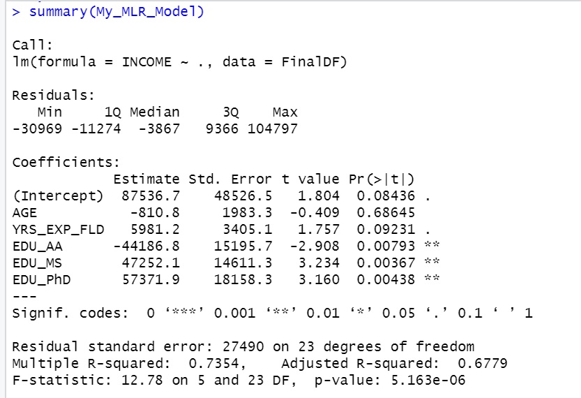
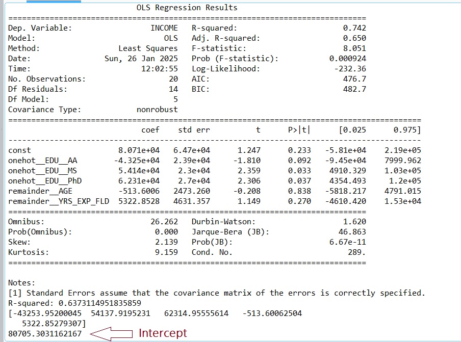
Below the image on the left offer the results from R and the image on the right offers the results from Python.
- Notice that while the intercept and coefficients calculated by R and by by Python are similar, they are not the same. This is because R and Python use different algorithmic methods and other underlying mathematical steps. We will not go into these details here, but it is important to understand any packaged algorithm you use.
Review, Discussion, and Analysis of R Results
(We leave the Python results analysis to the reader)
Part 1: Creating the Model
1.The R results illustrate the “Estimate” for the intercept as well as all five coefficients (weights) for our variables. We originally used the following definitions for our model: x1 as EDU_AA, x2 as EDU_MS, x3 as EDU_PhD, x4 as AGE, and x5 as YRS_EXP_FLD. The order that R presents the variables and their coefficient estimates does not control our designation of the order they appear in our Linear Model.
- However, it is required that the correct coefficient be associated with the correct variable. For example, here, we have x1 as EDU_AA. Therefore, the coefficient in front of x1 must be the coefficient for EDU_AA, which is -44186.8.
2. The Linear Model for this R output is:
y = -44186.8*x1 + 47252.1*x2 + 57371.9*x3 -810.8*x4 + 5981.2*x5 + 87536.7
Let’s plug in some values….
Suppose a person has an MS, is AGE 32, has 4yrs experience in the field
y = -44186.8*(0) + 47252.1*(1) + 57371.9*(0) -810.8*(32) + 5981.2*(4) + 87536.7
y = 132768 which is the income estimate from this model
Part 2: Interpreting the Linear Model Parameters
- Interpreting Quantitative Independent Variable Coefficients:
- When interpreting coefficients of quantitative independent variables in linear regression models that do not contain any categorical variables, any increase (or decrease) in the independent variable will directly effect the dependent variable. For example, a positive coefficient indicates a positive relationship and a negative coefficient indicates a negative relationship.
- Small Example where x1 and x2 are quantitative: y = 12×1 – 4×2 + 10 Here, for each “unit” x1 increases, the value of y will increase by 12. For each “unit” x2 increases, the value of y will decrease by 4. When x1 and x2 are both 0, the baseline value of y is 10.
- Interpreting Quantitative and Categorical Independent Variable Coefficients in a Mixed Model:
- When including categorical variables as dummy variables in a linear regression model, the dropped dummy variable is viewed as a baseline or reference level. It is part of the intercept, meaning its effect is incorporated into the constant term of the regression equation, not as a separate coefficient.
- This effects interpretation because all interpretations are now in reference to the dropped dummy.
- When a Linear Regression Model contains categorical independent variables, the “dropped” dummy variable (assuming one categorical variable) will join the intercept in forming the baseline. In addition, a change in a dummy variable will be relative to the baseline.
- The coefficient of a dummy variable represents the average difference in the dependent variable compared to the baseline/reference category (the “dropped” dummy variable), holding all other variables constant. This can be interpreted as “how much the dependent variable changes when the categorical variable switches from the baseline/reference level to the level represented by the dummy variable. Reference.
- We can think of this in simpler terms as – how much higher or lower the outcome is for that category compared to the reference category.
Examples Using Our Model
y = -44186.8*x1 + 47252.1*x2 + 57371.9*x3 -810.8*x4 + 5981.2*x5 + 87536.7
Let’s use the names of the variables to make this easier to think about: x1 as EDU_AA, x2 as EDU_MS, x3 as EDU_PhD, x4 as AGE, and x5 as YRS_EXP_FLD
y = -44186.8*(AA) + 47252.1*(MS) + 57371.9*(PhD) -810.8*(AGE) + 5981.2*(YRS) + 87536.7
(Note that the variables in the equation above are abbreviated for ease of reading.)
The dropped dummy is EDU_BS.
- Suppose all variable values, x1 through x5 are all set to 0. This tells us not only that the average income (the dependent variable value) is $87,536.70, but it also implies (per the dropped dummy) that this is for a BS degree.
- This almost makes sense – except for the AGE! It appears that one can make more than 87K per year at age zero.
- This is not uncommon when modeling, but there are methods such as “data centering” that can correct for odd outcomes like this. To learn more – here is a fun tutorial. Centering simply means subtracting the mean from the data.
- This almost makes sense – except for the AGE! It appears that one can make more than 87K per year at age zero.
- Suppose a person has an AA degree. How do we interpret the coefficients?
- Out model states:
- y = -44186.8*(AA) + 47252.1*(MS) + 57371.9*(PhD) -810.8*(AGE) + 5981.2*(YRS) + 87536.7
- Notice that the coefficient for AA is “-44186.8”.
- Recall that for our dummy variables (our categories) the coefficient is interpreted in relation to the dropped dummy. So, we can see that because the 44186.8 is a negative value, a person with an AA degree will make less income than our baseline reference point of Bachelors degree (BS) by about 44K.
- Suppose a person has a PhD. Here again, we relate the coefficient (57371.9) to the BS baseline. This tells us (holding all else) that a person with a PhD will make on average about 57K more than a person with a BS.
- Suppose a person has a BS and has 10 years of experience. How would be interpret this?
- In this case, because the person has a BS (which is our dropped dummy), we are saying that AA, MS, and PhD variables are all 0. Next, we also know the person has 10 yrs experience.
- From this, we can expect the income to be, on average, near to $147348.70 (without being able to take age into account). We also know that the age will reduce this value by $810.80 per year older. RE: y = -810.8*(AGE) + 5981.2*(10) + 87536.7
- As a final note, in all cases, because of the use of categorical variables and the dropped dummy (EDU_BS), all results are in reference to a person with a BS degree.
Part 3: Final Notes on the R Results
In reviewing the R results above, we can see that there are other measures given to us along with the coefficient and intercept estimates. The following will review each.
Std Error: “In a linear regression model in R, when variables are not standardized, the “standard error” refers to the residual standard error (RSE), which represents the average amount that the observed data points deviate from the fitted regression line; essentially, it’s the standard deviation of the residuals from the model, indicating how much error is expected on average in your predictions.” Reference.
“t value”: ” In a linear regression analysis in R, the “t-value” displayed for each variable in the model output represents the number of standard errors the estimated coefficient is away from zero, and this value is calculated using the unstandardized coefficients, meaning the variables do not need to be standardized to interpret the t-value; it reflects the significance of each variable in the model regardless of their original scale”. Reference.
“Pr(>|t|)”: “In a linear regression analysis in R, “Pr(>|t|)” represents the p-value associated with each regression coefficient, indicating the probability of observing a coefficient as extreme as the one calculated, assuming that there is no actual relationship between the predictor and response variables (null hypothesis); essentially, it tells you how likely it is to see such a result by chance, with a smaller value suggesting a stronger evidence against the null hypothesis and a more significant relationship between the variables.” Reference.
Extra Quick Note:
Variance Inflation Factor: “A Variance Inflation Factor (VIF) is a statistical measure used in regression analysis to quantify the degree of multicollinearity, or correlation between independent variables, within a model. It indicates how much the variance of a regression coefficient is inflated due to the presence of highly correlated predictor variables, making it harder to isolate the unique effect of each variable on the outcome.” Reference.
This is a rich topic and while this tutorial has come to an end, it is recommended that as a next step you research and consider methods to reduce multicollinearity, or correlation between independent variables.
It is also recommended that you review standardizing the non-dummy variables and how that might enable such things as ranking the coefficients.
Thank you for reading!
Dr. Ami Gates